Inhomogeneous matter distribution and supernovae
Version 1 Released on 20 May 2016 under Creative Commons Attribution 4.0 International LicenseAuthors' affiliations
- ICRANet
Keywords
Abstract
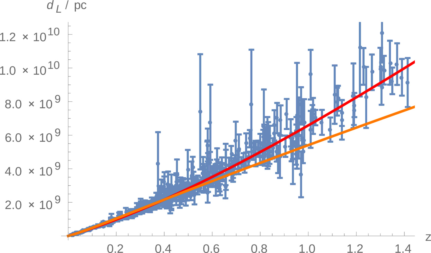
This work investigates a simple inhomogeneous cosmological model within the Lemaître-Tolman-Bondi (LTB) metric. The mass-scale function of the LTB model is taken to be $M(r) \propto r^d$ and would correspond to a fractal distribution for $0<d<3$. The luminosity distance for this model is computed and then compared to supernovae data. Unlike LTB models which have in the most general case two free functions, our model has only two free parameters as the flat standard model of cosmology. The best fit obtained is a matter distribution with an exponent of $d=3.44$ revealing that supernovae data do not favor those fractal models.
Introduction
The discovery that the observed peak luminosity of the IA supernovae (SNe IA) was smaller than the one implied by a $\Lambda=0$ Friedmann-Lema\^{\i}tre-Robertson-Walker (FLRW) model leads most of the scientific community to believe that our Universe was expanding at an increasing rate. To drive this expansion, an unknown perfect fluid $\Lambda$, dubbed dark energy, has been introduced by hand. Indeed a detailed fitting procedure, leads to the conclusion that the best-fit model is a flat FLRW metric filled with dark energy ($68 \%$) and pressureless matter ($32 \%$). This is called the concordance or $\Lambda$CDM model and is widely accepted and taught as the best candidate so far to describe our Universe. The very assumption of the $\Lambda$CDM model is that the geometry of our Universe is described by spatially homogeneous and isotropic spacetimes (called FLRW). Whereas statistical isotropy about our position has been established with a remarkable precision with the cosmic microwave background spectrum (CMB) observations,[1] statistical homogeneity on large scale is hard to probe mainly because it is hard to distinguish a temporal from a spatial evolution on the past light cone (two good reviews: Refs. [2,3]). This motivates to investigate more general spacetimes where the very assumption of statistical homogeneity is relaxed.
In the framework of Einstein's general relativity, a natural way to create an apparent acceleration is to introduce large-scale inhomogeneous matter distribution. This leads to many controversial philosophical debates (see eg. Ref. [4]). It has been shown that the Lemaître-Tolman-Bondi (LTB) [5–7] metric can successfully fit the dimming of the SNe IA by modeling radial inhomogeneities in a suitable way.[8,9] The fit of mass profiles to various datasets, including SNe, was performed for instance in Ref. [10]. The deduced acceleration of the expansion of the Universe induced by this unknown dark energy would be nothing but a mirage due to light traveling through an inhomogeneous medium, as explained eg. in Ref. [11]. However one caveat to these inhomogeneous LTB models is that under very mild assumptions on regularity and asymptotic behavior of the free functions of the LTB model, any pair of sets of conjugate observational data (for instance the pairs {angular diameter distance, mass density in the redshift space} or {angular diameter distance, expansion rate}) can be reproduced [12,13]. Proposing an alternative to the FLRW model which has so much freedom that it can fit any data sets seems problematic. Hence physical criteria are required to constrain the LTB models.
Then a data analysis is performed with the SNe IA data of Union2.1.[14] The result is that the data favor the flat FLRW model but the parametric LTB model fits also the data reasonably good. We argue that this model is interesting for two reasons. On the one hand, to show that a parametric LTB model can indeed fit SNIa data without dark energy even though it has much less freedom than the full general LTB model. On the other hand, to open the road to perform more broad and robust data analysis to check if indeed those classes of models can explain all the diverse cosmological data (CMB anisotropies and polarization, Integrated Sachs Wolfe effect, light element abundances, Baryon Acoustic Oscillation, Galaxies Surveys...) The paper is divided as follow, in section 2., we propose to discuss some of the theoretical and philosophical challenges for the homogeneous universes. Then we describe in section 3., the main ingredients of our parametric LTB model. The final goal of this section is to obtain an expression for the luminosity distance in the parametric LTB model. Then in section 4., a data analysis is performed to determined if this model can also account for the observed data of the SNe IA. A connection to fractal cosmologies is proposed in section 5.. Some concluding remarks and perspectives are drawn in section 6..
Homogeneity or inhomogeneity?
In this section, we posit some theoretical and philosophical thoughts on the choice of the FLRW metric to describe our Universe.
The observations of the CMB and galaxies surveys advocate for a universe statistically isotropic around us. Within these observations, usually one adds a principle to determine which class of cosmological solutions describes our Universe. The cosmological principle states that the Universe is spatially statistically homogeneous and isotropic. The Copernican principle is weaker and states that no observer has a peculiar position in the Universe. Combined with an isotropy hypothesis, the Copernican principle implies the cosmological principle. The cosmological principle is very ambitious because it conjectures on the geometry of the (possibly) infinite Universe whereas the Copernican principle applies only to the observable universe. Even though "principle" is an appealing wording, it reflects nothing but a confession of lack of knowledge on the matter distribution on large scale. Indeed, homogeneity cannot be directly observed in the galaxy distribution or in the CMB since we observe on the past lightcone and not on spatial hypersurfaces. An interesting study might be to consider this lack of knowledge in the context of the information theory and try to quantify how much information one can extract with idealized measurements and if this permits to draw any cosmological conclusion. Note[11] that FLRW models can only be called Copernician if one considers our spatial position. Considering FLRW models from a fully relativistic point of view: that is considering the observer in the four-dimensional spacetime, the model cannot be called Copernican. Indeed, whereas our position in space is not special, our temporal location is. Within the $\Lambda CDM$ model, this caveat is called the coincidence problem.
FLRW metric is the cosmological solution corresponding to a homogeneous and isotropic spacetime. Of course, the homogeneity and isotropy are valid up to some scale called the isotropic and homogeneity scale. On an epistemological point of view, it is unsatisfactory to have a model for a universe which is homogeneous but does not have any built-in prescription for its scale of homogeneity. A common order of magnitude for the homogeneity scale is hundred of Megaparsec but observations of larger and larger structures are being reported in the past decades (Ref. [15] for a recent example). Many people see them as Black Swan events but they could be more fundamental. It is furthermore interesting to note that the Hubble law is starting to be true when the proper velocity of the galaxy can be neglected ie. around 10 Mpc whereas the homogeneity scale is known to be much above ($\sim 100$ Mpc).
It has also been questioned whether the homogeneity assumption should be applied to Einstein tensor or the metric itself.[16] It is indeed known that in the general case $<G_{\mu \nu}(g_{\mu \nu})> \neq G_{\mu \nu}(<g_{\mu \nu}>)$, where $<...>$ denotes spatial average. This idea is really hard to implement because Einstein's equations are not tensor equations after the averaging procedure (changing from covariant to contravariant indices alters the equations). Then only tensors of rank 0 and scalars would have well behaved average [17]. The consequences of this approach are still unclear [18].
Describing our Universe with a FLRW spacetime does not tackle the so-called "Ricci-Weyl" problem. Ths usual FLRW geometry is characterized by a vanishing Weyl tensor and a non-zero Ricci tensor whereas in reality, it is believed that light is traveling mostly in vacuum where the Ricci tensor vanished and the Weyl is non-zero (see eg. Ref. [19] and references therein for more details). The parametric LTB models described in the next sections would be a possible extension of the Swiss-cheese models described in Ref. [19]. It would break the continuous limit and should reproduce more accurately the actual large-scale structure of our Universe (with voids and filaments).
The problems described previously are mainly gravitating around homogeneity assumption. Our current standard model of cosmology has many puzzling features: some fine-tuning problems, [20] the cosmological constant problem. [21] Inhomogeneous spacetime are less studied so their drawbacks are less known but they could give clues on the above mentioned problems.
LTB model:
The goal of this section is to derive an expression for the luminosity distance in a LTB model. To do so, we will first present some generalities about LTB model and then specify the class of models we will focus on. To connect to observations, the distances in LTB spacetime are presented and the final result for the luminosity distance is shown in Eq. \ref{eq:dl}.
LTB model: generalities
The model describes a spherically symmetric dust distribution of matter. In coordinates comoving with the dust and in synchronous time gauge, the line element of the LTB metric is given by: \begin{equation} \label{metric} ds^2=dt^2-\frac{R'^2(r,t)}{f^2(r)}dr^2-R^2(r,t) d\Omega^2. \end{equation} Our convention for derivatives are that a prime denotes a derivative with respect to the radial coordinate r and a dot a derivative with respect to cosmological time. $R(r,t)$ is the areal radius function, a generalization of the scale factor in FLRW spacetimes. It also has a geometrical meaning as it can be interpreted as the angular distance, as we will discuss in section 3.2.. $f(r)$ is the energy per unit mass in a comoving sphere and also represents a measure of the local curvature.
The time evolution of the areal radius function is given by the Einstein equation which reads: \begin{equation} \label{EOM} \frac{\dot{R^2}(r,t)}{2} - \frac{M(r)}{R(r,t)}= \frac{f(r)^2-1}{2}, \end{equation} where $M(r)$ is a second free function. After integrating (\ref{EOM}), one will find the third free function of the LTB model, namely $t_B(r)$ which is the bang time for worldlines at radius $r$. One will consider only a small class of LTB solutions. First the equations of the LTB model (\ref{metric}, \ref{EOM}) are invariant under the change of radial coordinate $r \rightarrow r + g(r)$ where $g(r)$ is an arbitrary function. This gives the possibility to choose one of the free function of the LTB model arbitrarily. The assumptions for these solutions are:
- The gauge freedom explained above allows us to choose one unique big-bang : $t_B(r)$ constant.
- We consider parabolic LTB solutions so that the geometry is flat: $f(r)=1$
- The free function $M(r)$ can be interpreted as the cumulative radius of matter inside a sphere of comoving size $r$ [7]. At this point, it is worth noting that a Einstein-de Sitter universe (flat, matter only, FLRW universe) is recovered for $M(r)=M_0 r^3$.
We choose the form of the free function $M(r)$ as following: \begin{equation} \label{condif} M(r)=\mathcal{M}_g N(r)= \mathcal{M}_g \sigma r^{d}, \end{equation} where $\mathcal{M}_g$ is the mass of a galaxy. This choice is our prescription to restrain the free function of the LTB models. $(\sigma, d)$ are two free parameters which will constrained by supernovae data. In section 5., a connection to fractal cosmologies will be described.
Observational distance
We will follow Ref. [22] for the definition of distances, more information and references can be found in that piece of work. Ellis [23] gave a definition of the angular distance which applied to the LTB metric gives $d_A=R$, one applies furthermore Etherington reciprocity theorem [24]: \begin{equation} \label{Th} d_L=(1+z)^2 d_A, \end{equation} which is true for general spacetime provided that source and observer are connected through null geodesics. Since, one considers a small class of parametric LTB model, an analytic solution of (\ref{EOM}) can be found: \begin{equation} \label{solu} R(r,t)= \left(\frac{9M(r)}{2}\right)^{1/3} (t_B+t)^{2/3}. \end{equation} Assuming a single radial geodesic [12], an analytical expression for the redshift as a function of the radial coordinate has been found in Ref. [22]: \begin{equation} \label{SNR} 1+z(r) = \frac{t_B^{2/3}}{(t_B+t)^{2/3}}=\frac{t_B^{2/3}}{(t_B-r)^{2/3}}. \end{equation} Using Eqs. (\ref{condif})(\ref{Th})(\ref{solu})(\ref{SNR}), it is possible to propose an expression for the parametric LTB luminosity distance: \begin{equation} \label{eq:dl} d_L=\left(\frac{9\sigma M_g}{2}\right)^{1/3} t_B^{\frac{d+2}{3}} \frac{\left((1+z)^{3/2}-1\right)^{d/3}}{(1+z)^{d/2-1}}. \end{equation} This will be the formula we will confront to its FLRW counterpart, it is only a function of the two parameters characterizing the matter distribution ($\sigma$,$d$). We will work with the following units: the unit of mass is $2.09\times 10^{22} M_{\odot}$, the time unit is $3.26\times 10^9$ years and the distances are given in Gpc. The big-bang time will be taken for the data analysis to be equal to 4.3.
Supernovae data analysis
In this section, we will fit the Union2.1 compilation released by the Supernova Cosmology Project [14]. It is composed of 580 uniformly analyzed SNe IA and is currently the largest and most recent public available sample of standardized SNe IA. The redshifts range is up to $z=1.5$
| parameter 1 | parameter 2 | $\chi^2$ | |
| flat FLRW | $\Omega_M=0.30\pm 0.03$ | $h=0.704 \pm 0.006$ | $538$ |
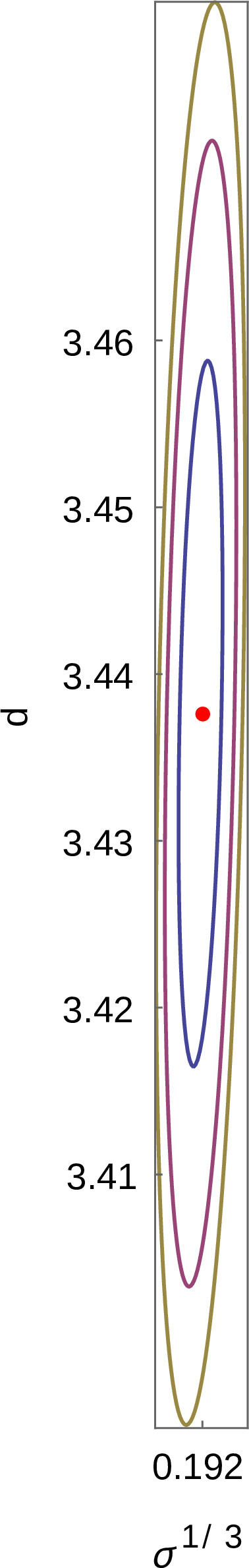
| parametric LTB | $d=3.44 \pm 0.03$ | $\sigma^{1/3}=0.192 \pm 0.002$ | $973$ |
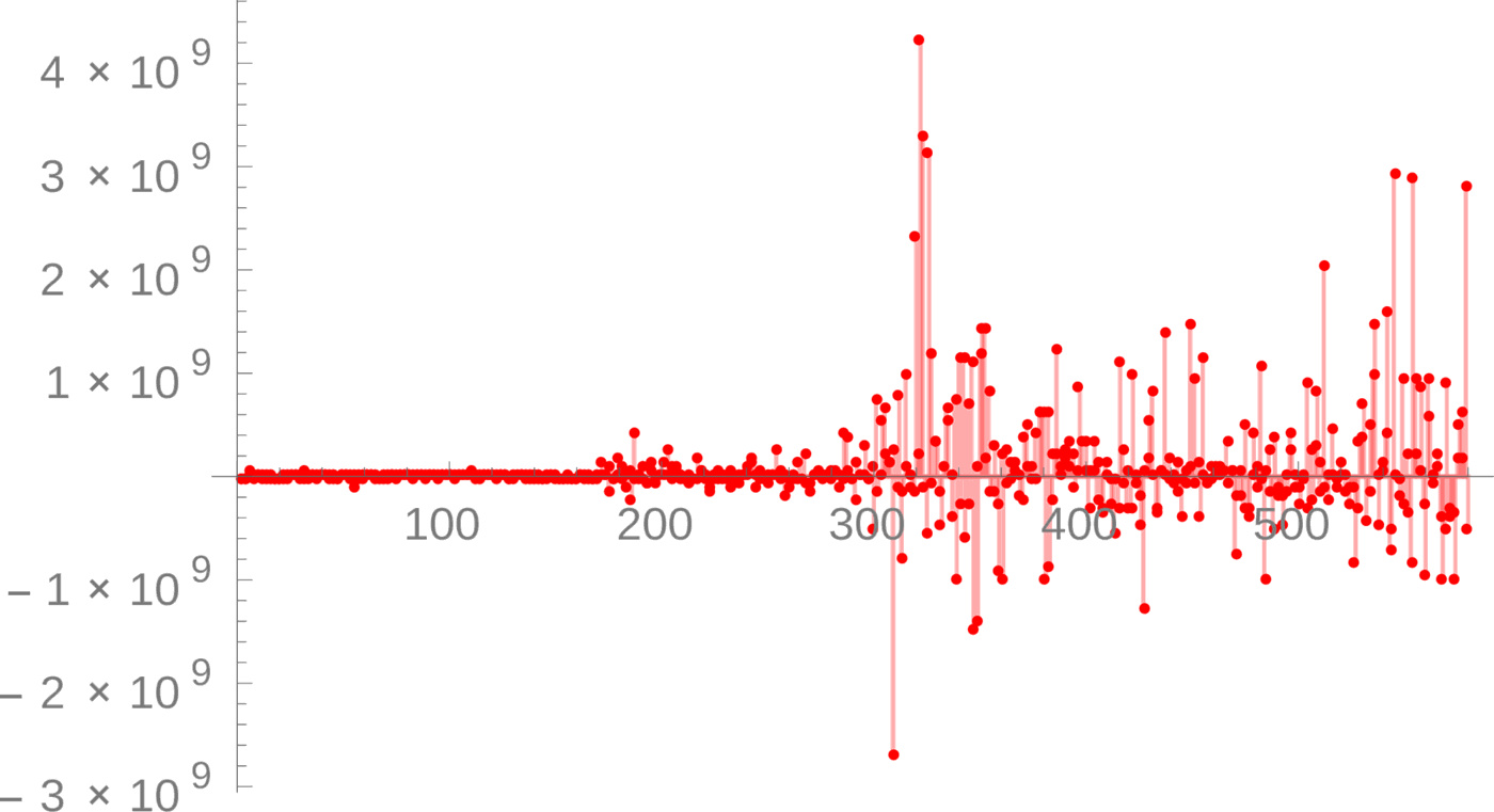
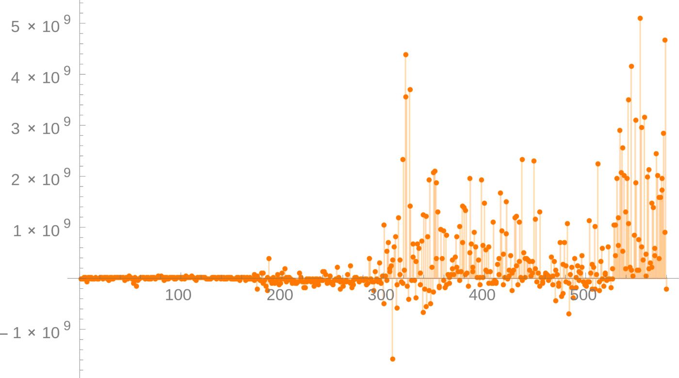
The shape of the SNe IA is empirically well understood but their absolute magnitude is unknown and need to be calibrated. One need either to analytically marginalize the assumed Hubble rate (or equivalently the absolute magnitude of the supernovae) [25], appendix C.2 of Ref. [26], or to use a weight matrix formalism (cf. Ref. [27]). Moreover, several authors pointed out the fact that the supernovae sample reduced with the SALT-II light-curve fitter from Ref. [28] are systematically biased toward the standard cosmological model and are showing a tendency to disfavor alternative cosmologies [29–31]. This might be an reason why the parametric LTB model fit has a bigger $\chi^2$.
A connection to fractal cosmologies
In this section, we will first review the use of fractal and explain how our model could be related to fractal matter distribution. The idea of fractals relies on spatial power law scaling, self-similarity and structure recursiveness.[32] These features are present in the formula: \begin{equation} N(r) \sim r^d, \end{equation} where $d$ is the fractal dimension, r the scale measure and N(r) the distribution which manifests a fractal behavior. If $d$ is an integer, it can be associated to the usual distribution (point-like for d=0, a line for d=1 and so on). The further from the spatial dimension, the more the fractal structure is "broken" or irregular. Note that topological arguments requires the fractal dimension to be smaller than the spatial dimension in which the fractal in embedded. This features of irregularity were useful to describe various structures from coastlines shapes to structure of clouds. In the context of cosmology, a fractal distribution would simply describe how clumpy, inhomogeneous our Universe is. Historically, this idea was popular in the late 80's,[33–35] then some more modern models were developed [36–38] and the relation to cosmological observation was also was worked out (see Refs. [39–41] and references therein for an analysis with galaxy distribution).
Using LTB models together with a fractal matter distribution has been already considered in Refs. [42–47]. In Ref. [22], following Ref. [33], the authors proposed a fractal inspired model by taking the luminosity distance as the spatial separation of the fractal ($N(r)=\sigma (d_L)^d$). This is motivated by the view of the fractal structure as an observational feature of the galaxy distribution. Since astronomical observation are carried out on the past null cone, the underlying structure of galaxy may not be itself fractal.[42,43]. The model proposed by Ref. [22] (and Ref. therein) is interesting but a clear problem appears, if one uses the self-similarity condition for the LTB model (Eq. (3.17)), it is clear that, at $z=0$, the mass function is not zero which is unsatisfactory (cf. also Fig. 3.5). In the same way, it can be shown that within the framework of Ref. [22], the luminosity distance is non zero at $z=0$, again this shows that this model cannot describe our Universe at low redshift.
The model we considered in the previous sections is such that $N(r)=\sigma r^d$ and could correspond to a fractal matter distribution if $0<d<3$ from topological considerations. The fractal is described by the coordinate $r$, that is the fractal structure is a geometrical effect which does not necessarily translate itself in an astronomically observable quantity. Contemplating the best fit of $d=3.44$ and within our working hypothesis, we can state that supernovae IA data do not support fractal models.
Conclusion and Perspectives
A parametric LTB model has been introduced in this work. It is characterized by two parameters ($\sigma$,$d$) like the flat FLRW model ($H_0$,$\Omega_M$). The link to SNIa data was then worked out leading to a comparison between the flat FLRW model and the parametric LTB model. The parametric LTB model can fit the data reasonably but the standard FLRW fit the data better. To keep testing such models, it is desirable to improve the data analysis with more elaborate techniques for SNe IA but also with others data sets eg. CMB anisotropies and polarization, Integrated Sachs Wolfe effect, light element abundances, baryon acoustic oscillation, Galaxies Surveys... One of the motivation to build such a model was to propose a physical input to constrain the general LTB where the two free functions that this model enjoys allow to fit any cosmological data under mild assumption on these free functions [12]. The parametric LTB model of this paper can be generalized to cases where $t_B(r)$ is not constant or (but not and because of the gauge freedom of the free functions of the LTB metric) by considering non uniformly flat geometries. It has been shown for instance in Ref. [48] that a nonsimultaneous big-bang can also account for the acceleration of the expansion of the Universe.
Since FLRW models are nowadays the most popular ones, many caveats of them are known and investigated with special care (cf. Sec. 2.). Even though, the LTB metric is less popular, some problems have also been identified and investigated. To account for the remarkable uniformity of the CMB observation, our location in the Universe has to be fine-tuned at (or close up to 1% to) the symmetry center of the LTB model [26] clearly violating the Copernican principle. Whether this fine-tuning is problematic is still debated nowadays:[11,49] for instance the FLRW model is also non-copernican from a fully-relativistic point of view. Another direction would be not to take LTB models too literally.[11,13] As for the FLRW, LTB models should be considered as a an approximation of the reality. In some average sense, it could be that an inhomogeneous metric captures the real world better than a perfectly symmetric one.[50] Other exact non spherically symmetric solutions exist, like the Szekeres model,[51,52] examples patching together FLRW and LTB metrics in a kind of Swiss cheese model,[53] patching Kasner and FLRW models,[19] meatball models.[54] Thus those models should not be taken as way to describe exactly our reality but as attempt to investigate inhomogeneous metric and see how much of our reality it grasps. Most of those extensions are in agreement with the Copernican principle.
When it comes to discuss structure formation in the FLRW model, one still assumes spatial homogeneity and isotropy but considers the forming structures as metric and matter perturbations. Performing the perturbation theory in a LTB metric is a really complex task, especially because a scalar-vector-tensor decomposition does not allow anymore to study separately the scalar, vector and tensor modes. Instead the "natural" variables to perform the perturbation theory give in the FLRW limit a cumberstone combination of scalars vectors and tensors. Efforts were done in this direction [55,56] but the perturbation techniques are not yet advanced enough to be challenged with realistic numerical simulations and observations as the FLRW model. In addition, the observation indicates the Universe to be very flat which created a fine-tuning problem christened the flatness problem. The solution for the FLRW universe was a period of inflation. Aiming at describing the early Universe with a LTB model, the same flatness problem might appear. However inflation would then occur differently in separate space location. This is a bizarre feature on which one can only speculates the consequences. It might be one different way to touch the multiverse scenario [57]. With a loss of generality for the free functions, it is always possible to demand the LTB model to approach the homogeneous limit in the early times, in which case the inflationary FLRW results apply [58].
To finish, all the models involving inhomogeneities do not solve the cosmological constant problem [21] but just shift it. From explaining a fairly unnatural value for it, one just assumes it is zero without providing any explanation. This is in complete disagreement with Loverlock theorem which states the cosmological constant appears naturally in any metric theory of gravity [59,60]. All the models of dynamical dark energy suffer from the same criticism.
Acknowledgments
The author expresses his gratitude to Vera Podskalsky for hosting him during the crucial part of this work. Disha Sawant, Gregory Vereshchagin and Remo Ruffini are also acknowledged for discussions. CS is supported by the Erasmus Mundus Joint Doctorate Program by Grant Number 2013-1471 from the EACEA of the European Commission.
References
- P. A. R. Ade et al. [Planck Collaboration], Astron. Astrophys. 571 (2014) A16 [arXiv:1303.5076 [astro-ph.CO]].
- R. Maartens, Phil. Trans. Roy. Soc. Lond. A 369 (2011) 5115 [arXiv:1104.1300 [astro-ph.CO]].
- C. Clarkson, Comptes Rendus Physique 13 (2012) 682 [arXiv:1204.5505 [astro-ph.CO]].
- G. F. R. Ellis, astro-ph/0602280.
- G. Lemaitre, Annales Soc. Sci. Brux. Ser. I Sci. Math. Astron. Phys. A47, 49 (1927).
- R. C.Tolman, Proc. Nat. Acad. Sci. 20, 169 (1934).
- H. Bondi, Mon. Not. Roy. Astron. Soc. 107, 410 (1947).
- M. N. Celerier, Astron. Astrophys. 353 (2000) 63 [astro-ph/9907206].
- H. Iguchi, T. Nakamura and K. i. Nakao, Prog. Theor. Phys. 108 (2002) 809 [astro-ph/0112419].
- S. Nadathur, S. Sarkar, Phys. Rev. D 83 (2011) 063506,
- M. N. Celerier, Astron. Astrophys. 543 (2012) A71 [arXiv:1108.1373 [astro-ph.CO]].
- N. Mustapha, C. Hellaby and G. F. R. Ellis, Mon. Not. Roy. Astron. Soc. 292 (1997) 817 [gr-qc/9808079].
- M. N. Celerier, K. Bolejko and A. Krasinski, Astron. Astrophys. 518 (2010) A21 [arXiv:0906.0905 [astro-ph.CO]].
- N. Suzuki et al., Astrophys. J. 746 (2012) 85 [arXiv:1105.3470 [astro-ph.CO]].
- L. G. Balazs, Z. Bagoly, J. E. Hakkila, I. Horvath, J. Kobori, I. Racz and L. V. Toth, arXiv:1507.00675 [astro-ph.CO].
- M. F.Shirokov and I. Z. Fisher, Soviet Ast. 6, 699 (1963).
- T. Buchert, Gen. Rel. Grav. 32 (2000) 105 [gr-qc/9906015].
- R. Zalaletdinov, Int. J. Mod. Phys. A 23 (2008) 1173 [arXiv:0801.3256 [gr-qc]].
- P. Fleury, H. Dupuy and J. P. Uzan, Phys. Rev. D 87 (2013) 12, 123526 [arXiv:1302.5308 [astro-ph.CO]].
- E. W. Kolb and M. S.Turner, The Early Universe (Addison-Wesley,1990), frontiers in Physics, 69.
- J. Martin, Comptes Rendus Physique 13 (2012) 566 [arXiv:1205.3365 [astro-ph.CO]].
- F. A. M. G. Nogueira, arXiv:1312.5005 [gr-qc].
- G. Ellis, Gen.Rel.Grav. 41, 581 (1971).
- I. M. H.Etherington, Phil.Mag. 15, 761 (1933).
- S. L. Bridle, R. Crittenden, A. Melchiorri, M. P. Hobson, R. Kneissl and A. N. Lasenby, Mon. Not. Roy. Astron. Soc. 335 (2002) 1193 [astro-ph/0112114].
- T. Biswas, A. Notari and W. Valkenburg, JCAP 1011 (2010) 030 [arXiv:1007.3065 [astro-ph.CO]].
- R. Amanullah et al., Astrophys. J. 716 (2010) 712 [arXiv:1004.1711 [astro-ph.CO]].
- J. Guy et al. [SNLS Collaboration], Astron. Astrophys. 466 (2007) 11 [astro-ph/0701828 [ASTRO-PH]].
- M. Hicken, W. M. Wood-Vasey, S. Blondin, P. Challis, S. Jha, P. L. Kelly, A. Rest and R. P. Kirshner, Astrophys. J. 700 (2009) 1097 [arXiv:0901.4804 [astro-ph.CO]].
- R. Kessler et al., Astrophys. J. Suppl. 185 (2009) 32 [arXiv:0908.4274 [astro-ph.CO]].
- P. R. Smale and D. L. Wiltshire, Mon. Not. Roy. Astron. Soc. 413 (2011) 367 [arXiv:1009.5855 [astro-ph.CO]].
- B. B.Mandelbrot, The Fractal Geometry of Nature (1982).
- L. Pietronero, Physica Rev. A 144 (1987).
- P. H.Coleman and L. Pietronero, Phys. Rept. 213, {311}(1992).
- R. Ruffini, D. Song, and S. Taraglio, Astron.Astrophys. 190 (1988).
- J. R. Mureika, JCAP 0705,021 (2007), gr-qc/0609001.
- Y. V. Baryshev, 'Practical Cosmology', v.2, pp.60-67, 2008 [arXiv:0810.0162 [gr-qc]].
- P. V. Grujic and V. D. Pankovic, arXiv:0907.2127 [physics.gen-ph].
- C. A. Chacon-Cardona and R. A. Casas-Miranda, Mon. Not. Roy. Astron. Soc. 427 (2012) 2613 [arXiv:1209.2637 [astro-ph.CO]].
- G. Conde-Saavedra, A. Iribarrem and M. B. Ribeiro, Physica A 417 (2015) 332 [arXiv:1409.5409 [astro-ph.CO]].
- J. S. Bagla, J. Yadav and T. R. Seshadri, Mon. Not. Roy. Astron. Soc. 390 (2007) 829 [arXiv:0712.2905 [astro-ph]].
- M. B. Ribeiro, Astrophys. J. 388 (1992) 1 [arXiv:0807.0866 [astro-ph]].
- M. B. Ribeiro, Astrophys. J. 395 (1992) 29 [arXiv:0807.0869 [astro-ph]].
- M. B. Ribeiro, Astrophys. J. 415 (1993) 469 [arXiv:0807.1021 [astro-ph]].
- F. Sylos Labini, M. Montuori and L. Pietronero, Phys. Rept. 293 (1998) 61 [astro-ph/9711073].
- F. S. Labini, Europhys. Lett. 96 (2011) 59001 [arXiv:1110.4041 [astro-ph.CO]].
- F. S. Labini, Class. Quant. Grav. 28 (2011) 164003 [arXiv:1103.5974 [astro-ph.CO]].
- A. Krasiński, Phys. Rev. D 89, 023520 (2014).
- P. Sundell and I. Vilja, Mod. Phys. Lett. A 29 (2014) 10, 1450053 [arXiv:1311.7290 [astro-ph.CO]].
- K. Bolejko and R. A. Sussman, Phys. Lett. B 697 (2011) 265 [arXiv:1008.3420 [astro-ph.CO]].
- P. Szekeres, Commun.Math.Phys. 41 (19 75) 55.
- K. Bolejko and M. N. Celerier, Phys. Rev. D 82 (2010) 103510 [arXiv:1005.2584 [astro-ph.CO]].
- T. Biswas and A. Notari, JCAP 0806 (2008) 021 [astro-ph/0702555].
- K. Kainulainen and V. Marra, Phys. Rev. D 80 (2009) 127301 [arXiv:0906.3871 [astro-ph.CO]].
- C. Clarkson, T. Clifton and S. February, JCAP 0906 (2009) 025 [arXiv:0903.5040 [astro-ph.CO]].
- A. Leithes and K. A. Malik, Class. Quant. Grav. 32 (2015) 1, 015010 [arXiv:1403.7661 [astro-ph.CO]].
- B. Carr, ed., Universe or Multiverse? (Cambridge University Press, 2007), ISBN 9781107050990.
- R. de Putter, L. Verde and R. Jimenez, JCAP 1302 (2013) 047 [arXiv:1208.4534 [astro-ph.CO]].
- D. Lovelock, J. Math. Phys. 12, 498 (1971).
- D. Lovelock, J. Math. Phys. 13, 874 (1972).
Footnotes
1. clement.stahl@icranet.org