The essential role of uncertainty and limited foresight in energy modelling
Version 1 Released on 25 April 2017 under Creative Commons Attribution 4.0 International LicenseAuthors' affiliations
- Geological Survey of Belgium – Royal Belgian Institute of Natural Sciences (RBINS)
Keywords
Abstract
When making techno-economic simulations to evaluate new climate mitigation technologies, a main challenge is to include uncertainty. The added level of complexity often causes uncertainties to be simplified or ignored in calculations, and not addressed in final public communications. This leads to inaccurate policy and investment decisions because probability is an essential aspect of assessing future scenarios. One specific source of uncertainty is the limitation of information available about the future, which is an aspect of everyday life, but simulation-wise a complex issue. It is however essential, because it is inherently tied to understanding semi-optimal decision making. Quite fundamentally, this pleads for stepping away from rather theoretical (partly) deterministic systems, and moving towards realistic limited foresight modelling techniques, such as offered by integrated Monte Carlo calculations.
Introduction
Climate change will have a lasting impact on society, and techno-economic modelling is performed to evaluate policy and investment decisions that aim to reduce its negative effects. Such simulations are future-oriented and typically include technologies that are not yet fully mature, such as next generation power plants or renewables and CO$_\mathrm{2}$ capture and storage (CCS), leading to important intrinsic uncertainty. Although a wide range of simulators and models are available, only a limited number of these are able to include uncertainties to some degree [1–5]. It is a striking observation that technology-related as well as other uncertainties seem insufficiently addressed in a societal debate where science plays a central role, especially when ignoring uncertainty leads to overconfident results and less than optimal scientific policy advice [6]. This is clearly demonstrated here with a new methodology that uses limited foresight principles for handling outlook uncertainty in techno-economic energy forecasting, that intrinsically shows that realistic quantification of the probability of forecasted results is, although challenging, often essential.
Most available models use an objective function or an optimization to provide an optimal result for a given scenario. A sensitivity analysis is then typically used in an attempt to map the robustness of the outcome in function of assumed inaccuracies on the forecasted input parameters, but inaccuracies due to non-optimal decision-making are implicitly ignored. The main outstanding challenge addressed here is making an energy model look forward in time while respecting the way the future is being shaped by the semi-optimal decisions that humans make, and the way uncertainty challenges the logic of such decisions. The real effect and the surrounding uncertainties may lead to results that are significantly different from a predetermined optimal scenario [3], which is an aspect that may easily prove essential when planning and preparing for the climate-energy nexus.
The workflow presented here enables the simulation of more realistic decisions in the context of energy modelling. Especially for technologies that are not yet mature, such as CO$_\mathrm{2}$ capture and storage (CCS), these simulations can deliver a clear first indication of the impact of this new technology on a nation's economy. The importance of uncertainties in general is underestimated or ignored, not only in the context of energy outlooks. Too often the average outlook is considered as the most important research result, while it may actually be the uncertainty ranges that contain the most valuable information. The latter, however, obviously requires an additional effort in obtaining, interpreting and presenting results, as well as in communicating their policy implications.
State of the art
The importance of uncertainty in climate-related modelling has been a point of discussion for decades. As uncertainty is inherent to forecasting, the correct confidence level of a certain prediction is essential when using such results for far-reaching policy decisions. This is why results of the IPCC Second Assessment Report [7] were criticised for not providing a quantitative indication of the uncertainties [8]. This concern was extensively addressed in the guidance documents for the third and following assessment reports, with a chapter devoted to quantifying uncertainty ranges [9]. Stein & Stein [6] describe convincingly the consequences of failing to consider actual uncertainties in geosciences with respect to natural hazards. The Fukushima Daiichi nuclear power plant for example proved to be insufficiently protected against the tsunami triggered by the 2011 Tôhoku earthquake. Here, the possible magnitude of an earthquake in that area was underestimated, causing a nuclear disaster.
Of direct importance for climate forecasting are the techno-economic models used for modelling energy systems and their environmental impact. Different families of modelling tools have been developed, each with their own characteristics [10]. In the frame of uncertainties, bottom-up models are of particular relevance. We will demonstrate the importance of limited foresight for making near-realistic simulations that address various sources of uncertainty, by looking in detail at the implementation of CCS in the energy system.
Many models that look at the impact of CCS technology are optimization models (e.g. MARKAL [11]). These models determine the optimal intermediate choices, in line with a given objective function, towards a future goal. These may for example be a sequence of technological choices to most economically reach a certain emission reduction target. The most essential point in the optimisation models is the objective function that is solved to find the optimal solution. Stochastic uncertainty that is resolved with time cannot be directly included in this type of models, except by introducing points in time when uncertainty is resolved [4]. These are, however, necessarily discrete, often only binomial bifurcations, such as an anticipated moment in time when worldwide climate consensus is assumed to be agreed or rejected, resulting in a predefined high or low carbon tax or emission standards from that moment on. Although these models have and will bring essential insights as optimised references, this significant abstraction of reality prevents them from being used as reliable forecasting tools. When considering techno-economic modelling of climate mitigation technologies with these optimization models, quantification of result probability is generally not being done, as uncertainties are dealt with by running different scenarios.
Less common models are simulation or forecasting models. These simulation tools do not optimise towards a set goal, but forecast starting from a set of start parameter values and simulate decision-making. These simulations can be compared to forecasting the behaviour of a physical, natural system such as the weather: the simulations start at a known state, and a set of processes determine how the system will behave towards the future. An advantage of forecasting over optimization models is that costs are not optimised, but are closer to costs in the real-world, as they try to mimic real market and human behaviour. Actual investment decisions are indeed rarely perfectly optimal, i.e. without the need of reversibility or change.
Investment decisions in the energy sector generally have an influence over several decades, and therefore shape the future, as much as they are susceptible to future changes. In order to model well-funded decisions, future projections and their uncertainties need to be taken into account. An important factor in modelling is the amount of information or type of foresight that is available at the moment of decision taking. The different approaches are crucial for simulating realistic decision-making. No foresight is the most basic form of foresight, in which it is assumed that only the information of today is available. On the other end of the spectrum lies perfect foresight, where it is assumed that the future is completely known (i.e. a deterministic system). In the latter case, a perfectly optimal investment decision can be taken, without the need to postpone decisions, or reassess further on in time. In technical terms, any parameter's uncertainty is resolved at the moment the investment decision is taken and the model knows the exact value of all parameters through time.
Reality lies somewhere in between no and perfect foresight: looking forward in time is like looking through a blurred pair of glasses: at close range details may still be identifiable, but what is further away is vague. This is referred to as limited or myopic foresight. Several attempts have been made to incorporate limited foresight in existing models to make projections more realistic. In the global energy model GET-LFL for example, optimization steps or decision horizons are shorter than investment lifetimes [1,2], and decisions can be revised after a certain amount of time. A comparable methodology is developed for the MESSAGE model, where Keppo & Strubegger [3] and Chen & Ma [5] describe a system with limited foresight by shortening the decision horizon, compared to the investment lifetime. When evaluating an investment decision, perfect foresight applies only for a limited period of time. This shortened decision horizon shifts along in time, and a re-evaluation of the investment decision is possible to adjust as new information becomes available.
Real options valuation is a methodology which, by considering investment (ir)-reversibility and parameter uncertainty, incorporates the possibility and value of project flexibility in an investment decision. Dixit & Pindyck [12] pioneered in this field by developing an analytical approach. For complex energy system simulations the analytical model quickly becomes unsolvable, and a numerical solution is preferable. Mathews et al. [13] for example present a Monte Carlo based solution as an alternative to a standard net present value calculation.
Here we propose a methodology, which forms part of the PSS simulator, a bottom-up techno-economic CCS simulator [14,15]. This is a methodology for limited foresight in techno-economic modelling that approaches reality and enables to look towards the future as investors or decision makers do: with an uncertainty that grows as forecasts extend forward in time, with imperfect decisions as a consequence. There is no model that includes limited foresight for techno-economic modelling in exactly this way.
Realistic limited foresight
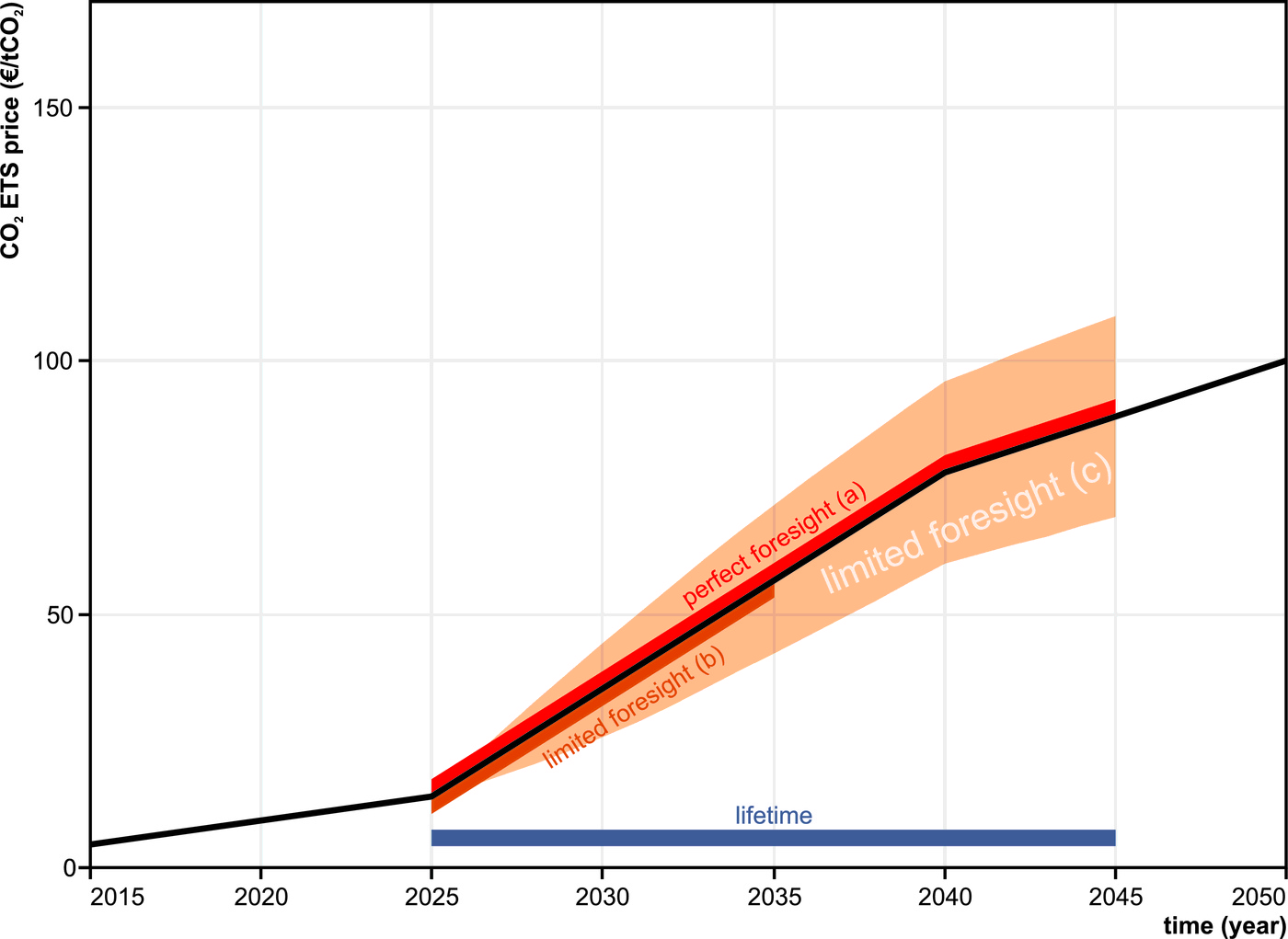
PSS has a standard Monte Carlo methodology to handle different stochastic parameters. Within a certain (primary) Monte Carlo calculation, the computer considers these stochastic parameter values as reality. Thus far, perfect foresight would apply: in a single Monte Carlo run, the best investment decision is found by calculating with actual parameter values that will occur over the decision horizon. In Figure 1, the red line shows an example of the CO$_\mathrm{2}$ price that is used for such a perfect foresight calculation, for an investment decision in the 2025 time step. For limited foresight as applied by Keppo & Strubegger [3], a restricted amount of information would be available in the 2025 time step (orange line in Figure 1). Note the difference in length of the decision horizon and the investment lifetime. In subsequent time steps, the decision horizon moves along. Based on the newly acquired information, the initial investment decision could then be changed.
In real life, one does not know the exact future value of a parameter, and decisions in simulations should be based on similarly imperfect information. The parameter uncertainty should only be completely resolved at a time that is considered as the present. In a typical case, uncertainty grows towards the future, producing a spectrum of possible outcomes, with the centre value being the most likely scenario. Such "fan charts" have been used and named first by the Bank of England in 1996 to illustrate uncertainty on their inflation forecasts [16] (see Section 4.).
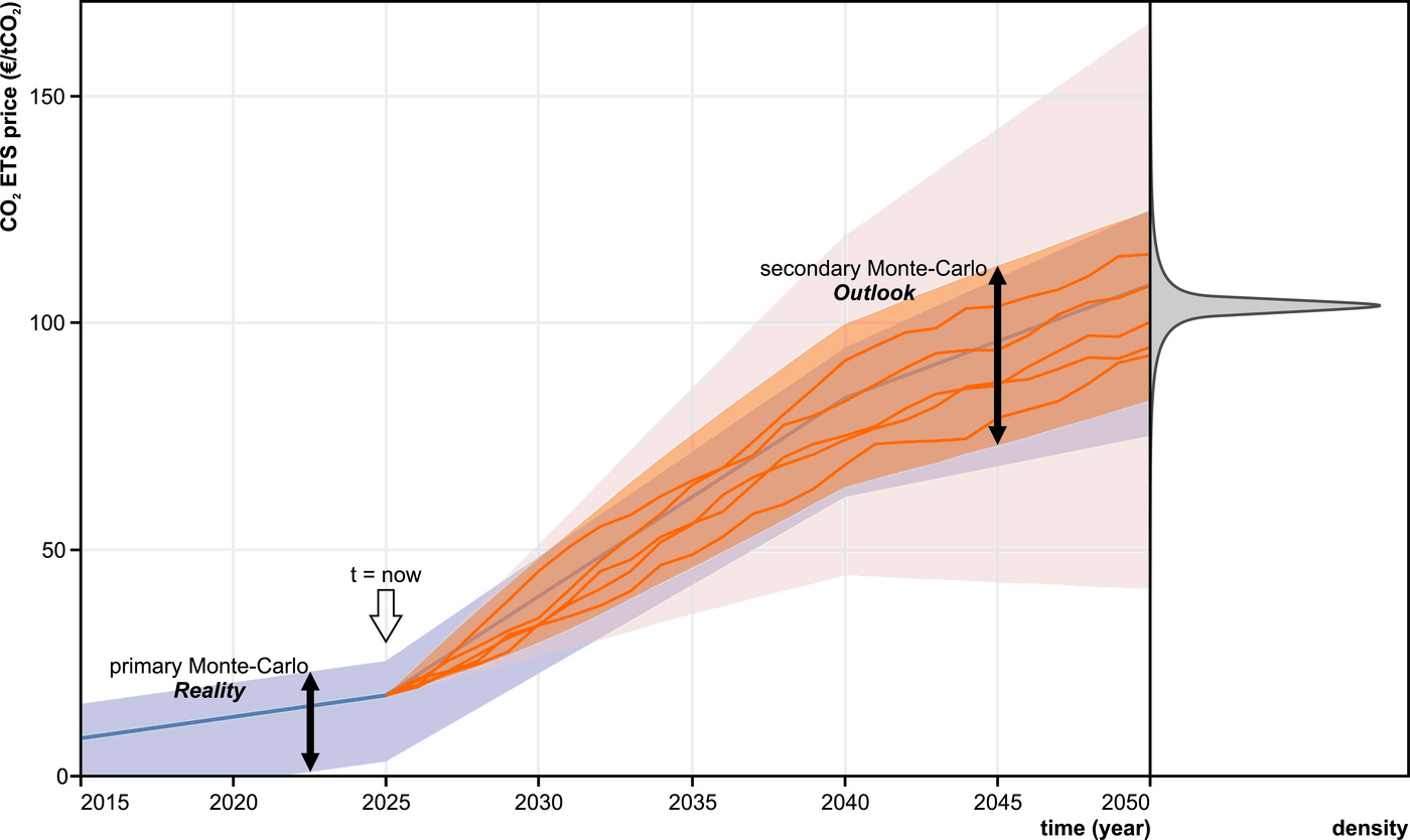
To mimic such a true myopic vision or growing uncertainty towards the future in simulations, we assume a growing range of possible "outlook" parameter values that lie around the actual value as an outlook uncertainty envelope (orange fan in Figure 1). This more realistic concept is parametrized into a model. The value of the current year is fixed (i.e. "reality", blue line in Figure 2). It is assumed that a parameter's value can rise or fall a fraction of a maximum value each year, starting from the previous year's value. This is a stochastic process, and can be categorised in-between a random walk and a one-dimensional Wiener process (equal to a Brownian motion in the natural world). In a random walk, both value and time axes are discrete. A Wiener process, however, requires both axes to be continuous. The process in our methodology has discrete time steps, but a continuous distribution on the value axis.
The upper and lower limits of this stochastic process produce a triangular envelope of possible outlook values (light grey area in Figure 2). To exclude unrealistic values from the limited number of Monte Carlo iterations that can be run, a percentile-limit can be imposed, which produces a funnel-shaped envelope (Figure 2, 90th percentile envelope in orange). Within this outlook envelope different random walks can be defined as possible parameter value pathways (Figure 2, orange lines).
Because of the nature of this stochastic process, the probabilistic distribution in a certain year approaches a normal density curve. This model mimics the fan charts of the Bank of England closely. Five stochastic processes are drawn for illustration. In order to make an informed investment decision next year, the uncertainty envelope will be shifted to a new origin, with the uncertainty range of each subsequent year being reduced.
In the approach of the PSS simulator, this secondary Monte Carlo simulation lies nested inside the primary Monte Carlo iteration. A project value will be calculated for every secondary Monte Carlo iteration using a single stochastic process. The result is a group of project value results, which can be analysed in a way that is appropriate for the simulation's goal. Unique to our methodology is that this is not the final simulation result. Simulated investment decisions will be based upon this data. This limited foresight principle is integrated in a decision tree and decisions are made with an adapted version of the modern portfolio theory, originally presented by Markowitz [18]. The investment decision that is made in a certain time step is thus based on a Monte Carlo analysis in which the outlook values of the parameter are used. These do not necessarily correspond to the actual modelled evolution of these parameters with time. Therefore, the decision taken cannot be the perfect, but will try to be close-to-optimal. In this way, PSS looks towards the future as if one would make a Monte Carlo analysis oneself to make an informed investment decision. This process of creating an outlook and making an informed close-to-optimal invest decision is repeated for the subsequent decision moments or years, until one primary Monte Carlo iteration is completed. Then the time line is reset, and a new primary Monte Carlo iteration is initialised with newly set stochastic parameters. In a nutshell, the primary Monte Carlo simulation defines what is regarded by the simulator as reality. In a single primary Monte Carlo iteration, investment decisions are taken based on the results of the secondary Monte Carlo simulation which provides an imperfect outlook.
Because of the law of large numbers, one would expect that running a sufficient number of Monte Carlo simulations would make the result converge towards an average or expected value. The degree of perfection with which investment decisions are taken can be controlled by limiting the number of secondary Monte Carlo iterations, whereby the calculated mean and variance, the two controlling parameters in the modern portfolio theory, can significantly differ from the centre or expected value and actual variance. When implemented into a decision tree, a certain fraction of non-optimal choices may result in substantial pathway differences and a discretisation of the output. The influence and importance of such results are discussed in the second part of this paper. This additional option to reduce the perfection of decision-taking to realistic levels also forms an important difference in comparison with a classical Real Options approach, where a truly optimal decision is taken, considering flexibility and risk.
The system of limited foresight as presented here (fan-shaped outlook) also offers additional flexibility. The uncertainty envelope has been described as having a symmetrical distribution around the central expected value of a parameter. By steering this envelope up or down, a more optimistic or pessimistic outlook is created, compared to what actually will happen during the simulated timeline (PSS "reality", further referred to as such). This means that the real parameter value will not be the expected value. This enables investigating the influence of unforeseen events in techno-economic simulations, for example a sudden market collapse, and especially how a given portfolio of choices will perform under unforeseen, and therefore non-optimal, conditions.
Fan charts and forecast probability density
A logical advancement from single-point forecasts, which do not include uncertainties, is the addition of an uncertainty range which grows as time progresses. This is usually expressed as a triangular or normal probability distribution around a centre, most probable value or mode. This approach produces a fan-shaped forecast region, leading to the first use of the term "fan chart" by the Bank of England for visualizing inflation rate and gross domestic product forecast probability. Such fan charts facilitate making financial decisions taking into account future uncertainty, or they can be used to present the uncertainty range associated with modelled results [16,19]. The main advantage of the fan chart is the ability of presenting the third axis of probabilistic data in a very intuitive way for interpretation. This enables easy communication, and valuable uncertainty information is less likely to be disregarded in communication with non-specialists.

In case of complex, nonlinear models, results will not have a linear or normal distribution; multimodal and strongly asymmetrical distributions are more common (see e.g. Figure 5). Hyndman [20] already mentions that such probabilistic density distributions are generally overlooked. Since then, forecasting and the processing and presentation of results have evolved much. Using the ggplot2 package for R for example, making complex density plots comes within everyone’s reach [21,22]).
Quantification of uncertainty
When considering techno-economic modelling of climate mitigation technologies, quantification of result probability is generally insufficiently performed or totally ignored. In assessing the effects of climate change, however, the importance of uncertainty quantification is recognised for years [23], and is still part of ongoing discussions [24]. Not every simulation methodology lends itself to produce result probabilities, and publishing these also requires a high level of confidence in the methodology used. Here we will not present a one-size-fits-all solution, but our intention is to show the importance of this aspect, which is eventually to have more realistic forecasting methodologies. This in turn will lead to better investment decisions and policy making, better tailored to answer to the different probable outlooks.
A methodology is needed which produces simulation results that enable a quantification of the uncertainty. As shown in the previous section, PSS is a forecasting simulator; its aim is to make forecasts that are as realistic as possible. As PSS is based on Monte Carlo calculations, the result is always a group of results, of which a density distribution can be made (PDF, probability density function), or a density mapping with time as a second axis. In this part, we will discuss a typical result of the PSS IV simulator to demonstrate the necessity and potential of quantitative uncertainty results from techno-economic simulations. Assuming that PSS produces realistic results, a density distribution of its results shows the probability that a certain scenario or event will happen in reality.
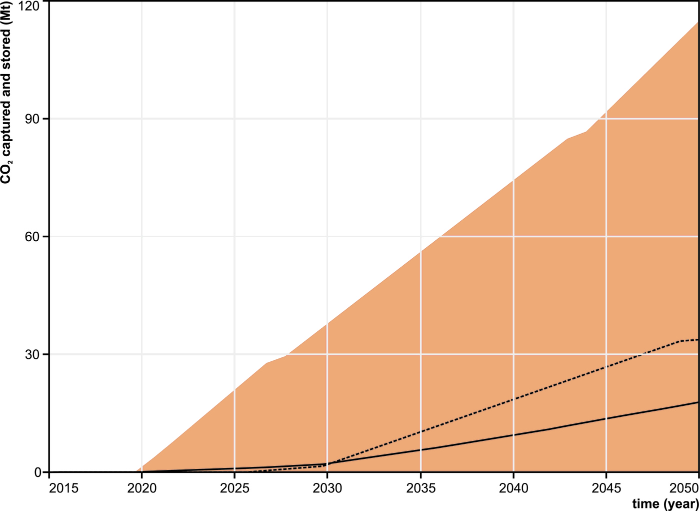
A simulation by PSS for Austria is used for illustrating the concern raised in this paper. The results presented here were obtained during the simulations shown in Welkenhuysen et al. [25]. The aforementioned paper focusses on the potential of geological reservoirs for storage of CO$_\mathrm{2}$ emissions from the power and iron & steel industry, but not on the emission quantities and technology choices which are used here to demonstrate the intrinsic importance that uncertainty and limited foresight play in energy modelling. Figure 4 shows the summarised results of 461 Monte Carlo iterations for the cumulative amount of CO$_\mathrm{2}$ captured from the iron and steel production industry, and stored in geological reservoirs between 2010 and 2050. The black line shows the average yearly value, and the red zone delineates the area between yearly minimum and maximum values. The width of the red zone shows that the average result is in no way representative for the whole result of possible future outcomes. On average, capture in significant amounts would start around 2030, while this could be as early as 2020 too. While on average 18 MtCO$_\mathrm{2}$ would be captured and stored until 2050, there is an uncertainty range of 0 to 115 Mt. This uncertainty envelope is already useful, but it does not allow for further quantification of probabilities, i.e. the likelihood of a certain scenario.
The average as shown here is a yearly mean value calculated over all Monte Carlo iteration results; it is not a single average Monte Carlo iteration result. In order to have an idea about what a single "average future" would look like, one non-stochastic simulation was run. All stochastic input values were fixed at their mean value. To maintain a certain realistic variety in the reservoir capacities, a random step was used in the fixation of their values. Limited foresight was still used. The non-stochastic result lies fairly high, at 34 Mt of CO$_\mathrm{2}$ captured and stored in 2050, much higher than the average value. This is possible because with the average input values, two iron & steel plants are equipped with capture technology, and there is no capture in the power sector. The limited amount of reservoir capacity can thus be used to its full extent by the iron and steel sector.
The true potential of the stochastic approach with limited foresight lies in its ability to quantify result probability. Results of the PSS calculations can be plotted as a density map (Figure 5). The probability density distribution in 2050 is given in grey. It is clear there is a preferred pathway (mode, pathway A), with capture staring after 2030 and having captured 7 MtCO$_\mathrm{2}$ in 2050. There is also a second likely future (B), with 25 Mt of CO$_\mathrm{2}$ captured and stored until 2050. In a third likely future (C), capture starts in 2020. In some cases capture ceases, which results in the shaded white and blue area. Looking at the overall picture, there is a 14% chance that over 30 MtCO$_\mathrm{2}$ is captured and stored, and 2% chance this amount is over 90 MtCO$_\mathrm{2}$. Equally, there is a 5% chance that no CO$_\mathrm{2}$ is captured in this timeframe. Each of the three scenarios represents the amounts of iron & steel production that are needed and produced by a discrete number of industrial plants, and their associated emissions which may be captured. The latter depends on the cost balance between traditional and capture technology and the availability of sufficient storage capacity.
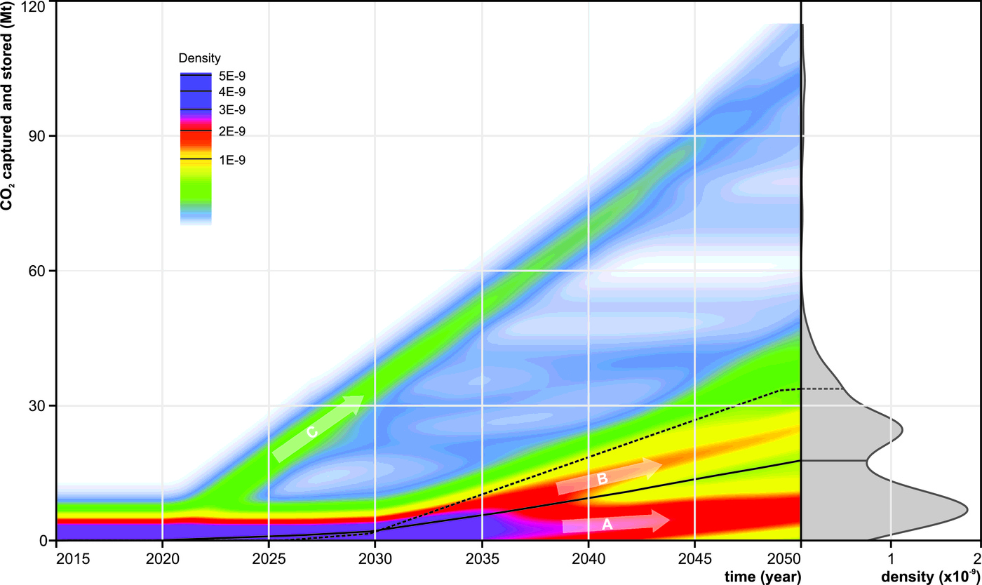
In Figure 5, the full black line again represents the yearly mean values, and the dashed black line shows the non-stochastic run, which is representative for a result that is obtained from a regular techno-economic simulation. Such average or single-run results are commonly used for further calculations or decisions, without considering the potential impact of uncertainty. From our analysis, it becomes clear that such an approach cannot be justified as in complex systems, where optionality forms a major factor in the decision process, an average scenario is in many cases not the most probable one. In case of the Austrian simulation, the average value falls right in between the two most likely scenarios, and in such a case it would be irresponsible to put all efforts on the average scenario.
With this example for CO$_\mathrm{2}$ storage in Austria it becomes clear that communicating uncertainties between research and policy is imperative for implementing realistic and credible climate change mitigation measures. An accessible and intuitive presentation of forecasting results helps improving communication at this interface (Section 4.).
The application of limited foresight in forecasting allows for a more realistic approach of risk and uncertainty. With the example presented here, we have demonstrated that uncertainty is more than a confidence interval around an average outlook. Instead, the outcome of a mature energy forecast will reflect the true risk, a truth which may entail that the most probable scenarios may substantially differ from the average result. This insight leads to the recognition that uncertainty quantification is essential in defining a realistic and credible climate policy. It is therefore our perspective that accepting risk, which is a major but well delineated part of the future, is one of the biggest mind shifts urgently needed to change the odds in the combat against climate change.
Acknowledgements
The foundations of the PSS methodology were developed during the PSS-CCS projects funded by the Belgian Science Policy Office (contracts SD/CP/04a&b and SD/CP/803). The simulations for Austria were made possible by financial support from the CGS Europe project exchange programme, funded by the European Union 7th Framework Programme (contract 256725). The authors also wish to thank Ed Garrett from the Royal Belgian Institute of Natural Sciences and Rudy Swennen from KU Leuven for providing valuable comments. Our gratitude also goes out to the numerous colleagues that were available for discussing our approach, and by doing so triggered continuous development over a little more than a decade now.
References
- B. Nyqvist. Limited foresight in a linear cost minimisation model of the global energy system, 2005.
- F. Hedenus, C. Azar, and K. Lindgren. Induced technological change in a limited foresight optimization model. The Energy Journal, 27:109–122, 2006.
- I. Keppo and M. Strubegger. Short term decisions for long term problems - the effect of foresight on model based energy system analysis. Energy, 35:2033–2042, 2010.
- R. Loulou and A. Lehtila. Stochastic Programming and Tradeoff Analysis in TIMES. Energy Technology System Analysis Programme (ETSAP), 2012.
- H. Chen and T. Ma. Technology adoption with limited foresight and uncertain technological learning. European Journal of Operation Research, 239:266–275, 2014.
- S. Stein and J. Stein. Playing against Nature: Integrating Science and Economics to Mitigate Natural Hazards in an Uncertain World. American Geophysical Union, 2014.
- IPCC. Climate Change 1995: A report of the Intergovernmental Panel on Climate Change. Second Assessment Report of the Intergovernmental Panel on Climate Change. IPCC, 1996.
- M.G. Morgan and D. Keith. Subjective judgements by climate experts. Environmental Science & Technology, 29:A468–A476, 1995.
- R.H. Moss and S.H. Schneider. Guidance Papers on the Cross Cutting Issues of the Third Assessment Report of the IPCC, chapter Uncertainties in the IPCC TAR: Recommendations to lead authors for more consistent assessment and reporting, pages 33–51. World Meteorological Organization, Geneva, 2000.
- A. Herbst, T. Felipe, F. Reitz, and E. Jochem. Introduction to energy systems modelling. Swiss Journal of Economics and Statistics, 148:111–135, 2012.
- R. Loulou, G. Goldstein, and K. Noble. Documentation for the MARKAL family of models. Energy Technology System Analysis Programme (ETSAP), Paris, 2004.
- A. Dixit and R. Pindyck. Investment under Uncertainty. Princeton University Press, Princeton, New Jersey, 1994.
- S. Mathews, V. Datar, and B. Johnson. A practical method for valuating real options: The boeing approach. Journal of Applied Corporate Finance, 19:95–104, 2007.
- K. Piessens, K. Welkenhuysen, B. Laenen, H. Ferket, W. Nijs, J. Duerinck, E. Cochez, Ph. Mathieu, D. Valentiny, J.-M. Baele, N. Dupont, and Ch. Hendriks. Policy Support System for Carbon Capture and Storage and Collaboration between Belgium-the Netherlands “PSS-CCS”, Final report. Belgian Science Policy Office, Research Programme Science for a Sustainable Development contracts SD/CP/04a,b & SD/CP/803, 2012.
- K. Welkenhuysen, A. Ramirez, R. Swennen, and K. Piessens. Ranking potential co2 storage reservoirs: an exploration priority list for belgium. International Journal of Greenhouse Gas Control, 17:431–449, 2013.
- E. Britton, P. Fisher, and J. Whitley. The inflation report projections: understanding the fan chart. Bank of England Quarterly Bulletin 1998 Q1, pages 30–37, 1998.
- European Commission. EU energy, transport and GHG emissions Trends to 2050: Reference Scenario 2013. Publications Office of the European Union, Luxembourg, 2013.
- H.M. Markowitz. Mean-Variance Analysis in Portfolio Choice and Capital Markets. Wiley, Milton Keynes, 1987.
- Bank of England. Inflation report - february 1996, 1996.
- R.J. Hyndman. Highest-density forecast regions for non-linear and non-normal time series models. Journal of Forecasting, 14:431–441, 1995.
- H. Wickham. ggplot2: Elegant Graphics for Data Analysis. Springer-Verlag New York, 2009.
- R Core Team. R: A Language and Environment for Statistical Computing. R Foundation for Statistical Computing, Vienna, Austria, 2014.
- J. Giles. When doubt is a sure thing. Nature, 418:476–478, 2002.
- M. Oppenheimer, C.M. Little, and R.M. Cooke. Expert judgement and uncertainty quantification for climate change. Nature Climate Change, 6:445–451, 2016.
- K. Welkenhuysen, A.-K. Brüstle, M. Bottig, A. Ramírez, R. Swennen, and K. Piessens. A techno-economic approach for capacity assessment and ranking of potential options for geological storage of co2 in austria. Geologica Belgica, 19:237–249, 2016.