Research article

An in-depth benchmark study of the CATE estimation problem: experimental framework, metrics and models

Version 1 Released on 10 June 2022 under Creative Commons Attribution 4.0 International License

Authors' affiliations

Square Research Center. Groupe Square

Keywords

Causal inference
Causal structure
Conditional average treatment effect
Randomised controlled trials
Rubin causal model
Synthetic datasets @Causal inference

Abstract

In the context of the Neyman-Rubin framework with binary treatment and outcome, we devise and conduct a rich benchmark study whose general ambition is to find the best practices to achieve good predictions of the CATE with machine learning techniques. The major part of our work revolves around two questions: i) what is the most reliable metric to select the best model among several competitors? We experimentally challenge the AUUC with the modified MSE associated with the AIPW pseudo-outcome, to which we introduce an alternative formulation. We compare them to multiple ground-truth-based metrics on synthetic datasets. ii) how do data generation processes impact the performance of models? We design a special structure for the benchmark and introduce axes of analysis to explore the global and local behaviours of several models (essentially neural nets and random forests). Beyond the validity of our conclusions, another important ambition of our work is to provide valuable data and methods to be included in the demanding and unified standard of model assessment we need to adopt as a research community in order to deepen our understanding of the CATE task and improve our models.

1. Introduction

We study randomized controlled trials with a binary treatment and a binary outcome. A population is randomly divided into two groups and only one receives the treatment. The negative or positive outcome of this assignment policy is then observed at the individual level. Our goal is to ascertain the causal effect of the treatment for any particular profile. How likely is an individual with given characteristics to benefit from the treatment? Will treating him/her change his/her natural course?

Being able to answer this question opens up a large field of applications. In the medical domain, it may considerably strengthen the therapeutic armamentarium by going beyond the standard analysis that only assesses the overall efficiency of a treatment. Indeed, even if a treatment displays a weak average effect, the comprehensive identification of the profile-based response of patients might still reveal that it is an efficient solution for a specific subset of the population. In marketing, it would allow to accurately target customers that are prone to buy a product, improving the company's return on investment while reducing the amount of spamming from the consumer's perspective. For example, it has been used in Barack Obama's campaign in order to target passive supporters likely to be persuaded to go to the polling station and vote on election day, with apparent success.

We are practitioners interested mainly in the applications of causal inference to marketing using machine learning techniques. In this article, we report all of our work, ideas and findings that originated from the question: what is, in practice, the best machine learning model for the problem? The answer we are looking for is of experimental nature and led us to thoroughly consider aspects that are generally secondary in state of the art articles, which introduce, for instance, new models. Precisely, we focus on two fundamental questions:

How to compare models with each other and select the best one? We considered alternatives to the standard metric of the field (the AUUC) and designed an experimental way to compare their merits.
How to test the models and better understand their strengths and weaknesses? We designed a challenging benchmark and introduced a way to analyze the local behaviour of models. Throughout this process, we also make our own propositions in terms of metrics and models.

We developed all the code in Python, which is publicly available at https://github.com/SRC-data/uplift_adway.

Because of the diversity of causal inference applications and the way scientific publishing is organized, the topic is unfortunately scattered throughout many different fields under different names. However, to the best of our understanding, there is no field-induced specificity of the problem that could justify such a siloed situation. Consequently, the state-of-the-art is hard to monitor and it slows down the diffusion of ideas between fields. In this article oriented towards experimentation, we aim to lay the foundation of a cross-field experimental standard for the topic, which may interest all its contributors. We are already aware of some improvements to our proposals, and we are inevitably ignorant of others since the literature is vast. We, therefore, hope that this article will be the vehicle of a collective discussion resulting in a global consensus about experimental standards, whether the ones we propose initially or not, for science's sake.

1.1. Set-up and notations

We work with a dataset in which every individual, besides his features, has two labels denoting whether he received the treatment and the observed outcome. We denote:

$X$ the $\Omega$-valued random variable ($\Omega \subset \mathbb{R}^d$) representing the features of an individual.
$T$ the treatment label, $T=1$ meaning the treatment has been assigned and $T=0$ otherwise.
$Y$ the outcome label, $Y=1$ meaning the positive outcome has been observed and $Y=0$ otherwise.

We denote respectively $Y_i(1)$ and $Y_i(0)$ the outcomes that would be observed if the treatment was assigned or not to the individual $i$. $\{Y_i(0), Y_i(1)\}$ fully defines the effect of the treatment on the individual $i$ and we have $Y_i = T_i Y_i(1) + (1-T_i)Y_i(0)$.

We refer to the population group of treated individuals as the test population and the rest as the control population.

We denote $w(x)$ the propensity, the probability to assign the treatment to individuals of profile $x$: $w(x) = P(T=1|X=x)$.

We denote $\mu_1(x)$ and $\mu_0(x)$ the response surfaces, i.e. $\mathbb{E}[Y(1)|X=x]$ and $\mathbb{E}[Y(0)|X=x]$.

We denote $N$, $N_T$ and $N_C$ the size of the dataset, of the test population and of the control population ($N=N_T+N_C$).

In the following, unobservable quantities will be displayed in green.

1.2. The ideal task: deriving the causal structure of a dataset

In this section, we want to highlight what we coin the causal structure of a dataset. Deriving the causal structure of a dataset leads, in our opinion, to the highest level of understanding of the causal effect of the treatment. Importantly, this objective is not the one that will be pursued in the rest of the article. However, it emphasizes an underlying structure of the problem that will be yet useful in interpreting the results and in the design of our benchmark.

The causal structure is a specific concept to the case of binary treatment and outcome. Here, individuals fall into one of four mutually exclusive categories which fully describes their behaviour:

Individuals such that $\{Y_i(0), Y_i(1)\} = \{0,1\}$ are called responders (R). They benefit from the treatment, i.e. the positive outcome happens only when they have been treated.
Individuals such that $\{Y_i(0), Y_i(1)\} = \{1,1\}$ are called survivors (S). The treatment does not affect their behaviour and they always display a positive outcome.
Individuals such that $\{Y_i(0), Y_i(1)\} = \{0,0\}$ are called doomed (D). The treatment does not affect their behaviour and they always display a negative outcome.
Individuals such that $\{Y_i(0), Y_i(1)\} = \{1,0\}$ are called anti-responders (A). The treatment has a deleterious effect on them: they display a positive outcome only when they are not treated.

These categories form a partition of the dataset: any population can be described as a mixture of these four causal sub-populations. Denoting $\textcolor{green}{\pi_k}$ their relative abundance and $\textcolor{green}{f_k(x)}$ their distribution (with $k \in \{R,S,D,A\}$), we have $P(X=x) = \textcolor{green}{\pi_R f_R(x)} + \textcolor{green}{\pi_S f_S(x)} + \textcolor{green}{\pi_D f_D(x)} +\textcolor{green}{\pi_A f_A(x)}$. We define then the causal structure of a dataset $\textcolor{green}{\mathcal{C}}$ as: \begin{equation} \textcolor{green}{\mathcal{C}} = \textcolor{green}{\{(\pi_R,f_R), (\pi_S, f_S), (\pi_D, f_D), (\pi_A, f_A)\}}. \end{equation} We consider that the explicit knowledge of $\mathcal{C}$ constitutes the highest level of representation of the causal information, from which all other quantities of interest can be computed and interpreted.

1.3. The CATE problem

In this article, we focus on determining the optimal and individual treatment assignment policy. Let us consider a marketing application where it costs $c(x)$ to advertise a product of price $q(x)$ to customers of characteristics $x$. A customer should be treated if the gain $\textcolor{green}{G(1)}$ when treated is expected to be greater than the gain $\textcolor{green}{G(0)}$ when not treated. We have: \begin{eqnarray} \textcolor{green}{\mathbb{E}[G(1)|x]} &=& q(x)\textcolor{green}{\mathbb{E}[Y(1)|x]}-c(x)\nonumber\\ \textcolor{green}{\mathbb{E}[G(0)|x]} &=& q(x)\textcolor{green}{\mathbb{E}[Y(0)|x]}\nonumber\\ \textcolor{green}{\mathbb{E}[G(1)|x]} &>& \textcolor{green}{\mathbb{E}[G(0)|x]} \Rightarrow \textcolor{green}{\mathbb{E}[Y(1)|x]}-\textcolor{green}{\mathbb{E}[Y(0)|x]} > c(x)/q(x) \label{eq:CATE_pratique} \end{eqnarray}

Thus, the optimal assignment policy boils down to the estimation of the quantity: \begin{equation} \textcolor{green}{\tau(x)} = \textcolor{green}{\mathbb{E}[Y(1)|x]}-\textcolor{green}{\mathbb{E}[Y(0)|x]}, \label{eq:def} \end{equation} followed by the selection of individuals for whom $\tau$ is greater than a certain threshold.

This quantity was introduced first by (Rubin 1974 [1]) in the Journal of Educational Psychology under the name of causal effect. Since then, it has spread across many different fields (such as epidemiology, econometrics, marketing, statistics or machine learning) under different names: conditional average treatment effect, individual treatment effect, heterogeneous treatment effect, uplift, net score, incremental response, etc. In this article, we will use the conditional average treatment effect (CATE) as the reference name for $\textcolor{green}{\tau}$, since we consider it describes better its standard expression \ref{eq:def}.

As suggested in the previous subsection, though, the causal structure perspective could shed new light on the CATE and provide another interpretation, from which yet another name could be derived. Indeed, by marginalizing over the causal populations, we have:

\begin{eqnarray*} \textcolor{green}{\mathbb{E}[Y(1)|x]} &=& \textcolor{green}{\mathbb{E}[Y(1)|x,R]}\times \textcolor{green}{p(R|x)} + \textcolor{green}{\mathbb{E}[Y(1)|x,S]}\times \textcolor{green}{p(S|x)} \\ &&+ \textcolor{green}{\mathbb{E}[Y(1)|x,D]}\times \textcolor{green}{p(D|x)} + \textcolor{green}{\mathbb{E}[Y(1)|x,A]}\times \textcolor{green}{p(A|x)} \\ &=& 1 \times \textcolor{green}{p(R|x)} + 1 \times \textcolor{green}{p(S|x)} + 0 \times \textcolor{green}{p(D|x)} + 0 \times \textcolor{green}{p(A|x)}\\ &=& \textcolor{green}{p(R|x)} + \textcolor{green}{p(S|x)}. \\ \textcolor{green}{\mathbb{E}[Y(0)|x]} &=& \textcolor{green}{p(S|x)} + \textcolor{green}{p(A|x)} \textrm{\ \ similarly}. \end{eqnarray*} So that: \begin{equation} \textcolor{green}{\tau(x)} = \textcolor{green}{p(R|x)} - \textcolor{green}{p(A|x)}. \label{uRSDA} \end{equation} Thus, the CATE can also be understood as the local difference between causal population densities.

1.4. Assumptions

In this study of the CATE, we require the following points:

we assume unconfoundedness $\{Y(0),Y(1)\} \perp T|X$. Under this condition, we can identify the response surfaces: we have $\mu_1(x) = \mathbb{E}[Y=1|T=1,x]$ and $\mu_0(x) = \mathbb{E}[Y=1|T=0,x]$. This assumption also implies that each causal population is equally distributed between the test and control populations. This assumption is guaranteed in randomized controlled trials but not in observational studies.
we assume that $0<w(x)<1$: we restrict the study of the CATE to the region where observations are available for both the test and control populations.
we also assume SUTVA (stable unit treatment value assumption), which requires that each sample $i$ is not affected by the treatment received by other samples.
last, we assume that the propensity $w(x)$ is explicitly known. This is undoubtedly wishful thinking in the context of medical data which mostly come from observational studies, but it is likely for marketing applications where marketers can freely plan their targeting strategy. In the general case where the propensity is unknown, an estimate of the propensity $\hat{w}(x)$ needs to be computed first, and it should replace every occurrence of $w(x)$ in what follows.

2. Review of the state of the art

We want to review three aspects of state of the art: the metrics of the problem, the models and the experimental set-up.

2.1. Metrics

A fundamental difficulty of the problem is that it is impossible to observe {$Y_i(0),Y_i(1)\}$ for an individual $i$: treating him and thus “revealing” $Y_i(1)$ prevents us to ever observe $Y_i(0)$, i.e. to know what would have happened if we had not treated him. We therefore cannot know his class for certain: we rather always face an undecidable choice between two classes. For instance, if we know that $Y_i(1)=0$, we can be sure that $i$ is neither an anti-responder nor a survivor, but cannot decide whether he is a responder or a doomed. Similarly, $\tau(x_i)$ cannot be observed. In terms of machine learning, this difficulty is reflected in the design of a metric.

2.1.1. Wishlist for a metric

Let us start by laying down what we consider the desirable properties of a metric $\mathcal{M}$ for the CATE problem:

Calibration: the ground truth should achieve the optimal score, i.e. $\tau = \operatorname*{arg\,max}_{\hat{\tau}} \mathcal{M}(\hat{\tau})$. Thus, improving the score of a prediction indeed implies that it is somewhat closer to the ground truth and is a worthy goal indeed.
Rewarding correct CATE values: as shown in \ref{eq:CATE_pratique}, the user decides the assignment policy by comparing the CATE with a certain threshold. Thus, the metric should guarantee that CATE estimations are correct.
Differentiability The metric should be differentiable so that a robust optimization process can be designed. Additionally, it should have good smoothness properties.

Then, this metric would be ideally used at three stages of the machine learning framework:

as an objective function for model training,
as a relative measure of the performance of trained models that enables comparison and selection of the best ones,
and as an absolute measure of performance of selected models that will make sense to their end users.

2.1.2. The Area Under the Uplift Curve (AUUC)

Introduced in [2] as a natural extension of lift curves to the CATE problem, the Area Under the Uplift Curve (AUUC) is the most common metric used in the literature, also referred to as Qini coefficient. It aims at assessing whether a prediction ranks the samples correctly. The general idea is to maximize the area under the curve obtained when subtracting the lift curves (i.e. the cumulative fraction of positive outcomes detected as we treat samples in decreasing order of predicted CATE) drawn respectively on the test and the control populations. Some minor variations in its definition can be found in the literature (see [3] for a summary). Here we will work with the definition used in [4]. Be $\Gamma_k(\hat{\tau})$ the set of the $k$ first samples of the highest CATE as predicted by a model $\hat{\tau}$. Then : \begin{eqnarray} AUUC(\hat{\tau}) &=& \sum_{k=1}^{N} V(\hat{\tau},k) \\ \mathrm{with \ \ }V(\hat{\tau},k) &=& \sum_{i \in \Gamma_k(\hat{\tau})} Y_i\left(\frac{T_i}{N_T} - \frac{1-T_i}{N_C}\right) \end{eqnarray}

How does the AUUC fare with the wishlist of the previous subsection (2.1.1)?

Rewarding correct CATE values — The AUUC is a rank metric. If $\hat{\tau}$ is an estimator of the CATE, any transformation $f(\hat{\tau})$ where $f$ is an increasing function will have the same AUUC as $\hat{\tau}$. Therefore, it does not provide the guarantees the user expects in order to achieve optimal assignment policy.

Calibration — The AUUC is calibrated in the limit of a large number of samples [5]. There is no reason why it is calibrated in the general case and our benchmark does provide examples where the trained model $\hat{\tau}$ is such that $AUUC(\hat{\tau}) > AUUC(\tau)$. As far as we know, the convergence of the AUUC has not been theoretically studied.

Differentiability — The AUUC is not differentiable.

Therefore, the standard use of the AUUC in the field can be challenged. Different ideas that could be used as alternatives already stem in the literature, and we want to shortly discuss them.

2.1.3. IPW pseudo-outcome and modified MSE

This idea stems from the literature on the average treatment effect (ATE), defined as $\mathbb{E}[Y|T=1] - \mathbb{E}[Y|T=0]$. Horvitz and Thompson [6] showed in 1952 that the ATE could be estimated through the so-called IPW (inverse propensity weighting) estimator: \begin{eqnarray*} \hat{ATE}_{IPW} &=& \frac{1}{N}\sum Y^*_i \\ \mbox{with \ } Y^{*}_i &=& Y_i(\frac{T_i}{\hat{w}_i} - \frac{1-T_i}{1-\hat{w}_i}) \end{eqnarray*} In [7], Athey et al. notice that $Y^*$ is an unbiased estimator of the CATE, i.e. $\mathbb{E}[Y^*|x]=\tau(x)$, so that $Y^*$ is a pseudo-outcome that could be “repurposed” as a target for regressors in lieu of $\tau$. In particular, the authors focus on the “modified MSE” metric: \begin{equation} \hat{\mathcal{L}}(\hat{\tau}) = \frac{1}{N}\sum(\hat{\tau}(X_i)-Y^*_i)^{2}. \label{TOT} \end{equation}

Calibration — As the AUUC, the modified MSE is asymptotically calibrated. Indeed, the modified MSE and the true MSE, defined as: $\textcolor{green}{\mathcal{L}(\hat{\tau})} = \textcolor{green}{\frac{1}{N}\sum(\hat{\tau}(X_i)-\tau(X_i))^{2}}$, relate in the following way:

\begin{eqnarray} \hat{\mathcal{L}}(\hat{\tau}) &=& \frac{1}{N}\sum((\hat{\tau}(X_i) - \textcolor{green}{\tau}(X_i)) +(\textcolor{green}{\tau}(X_i)- Y^*_i))^{2}\\ &=& \textcolor{green}{\mathcal{L}}(\hat{\tau}) - \frac{2}{N}\sum \hat{\tau}(X_i)(\textcolor{green}{\tau}(X_i)-Y^*_i) + \textcolor{green}{C}, \label{eq:L} \end{eqnarray} where $\textcolor{green}{C}$ is a term that depends only on the dataset and the DGP (data generation processes). The second term is asymptotically zero. Indeed: \begin{equation} \frac{1}{N}\sum \hat{\tau}(X_i)(\textcolor{green}{\tau}(X_i)-Y^*_i) \rightarrow \mathbb{E}[\hat{\tau}(\textcolor{green}{\tau}-Y^*)] \\ \end{equation} \begin{eqnarray*} \mathbb{E}[\hat{\tau}(\textcolor{green}{\tau}-Y^*)] &=& \mathbb{E}[\mathbb{E}[\hat{\tau}(\textcolor{green}{\tau}-Y^*)]|X] \\ &=& \mathbb{E}[\hat{\tau}(X)\mathbb{E}[\textcolor{green}{\tau}-Y^*|X]] \mbox{\ since\ } \hat{\tau} \mbox{\ is just a function of X}\\ &=& \mathbb{E}[\hat{\tau}(X) \times 0] = 0. \end{eqnarray*} Thus, $\hat{\mathcal{L}}$ allows to select the true model $\textcolor{green}{\tau}$ in the limit of a large number of samples. The quality of $\hat{\mathcal{L}}$ as an approximation of $\textcolor{green}{\mathcal{L}}$ depends on how fast the term $\frac{1}{N}\sum \hat{\tau}(X_i)(\textcolor{green}{\tau}(X_i)-Y^*_i)$ converges to zero.

It is clear that the ground truth is not the optimum of the modified MSE in the general case: it would imply that $Y^*$ is actually a perfect estimator, i.e. $Y^*|X = \tau(X)$.

Rewarding correct CATE values — The focus of the modified MSE is indeed on CATE values.

Differentiability — The modified MSE is differentiable.

2.1.4. AIPW pseudo-outcome

Introduced in [8], the AIPW estimator (for “augmented IPW”) is a pseudo-outcome that relies on a preliminary estimation of the response surfaces $\hat{\mu}_1$ and $\hat{\mu}_0$. It is defined as: \begin{equation} \phi^*_i = \hat{\mu}_1(x_i) - \hat{\mu}_0(x_i) + T\frac{Y-\hat{\mu}_1(x_i)}{\hat{w}(x_i)} - (1-T)\frac{Y-\hat{\mu}_0(x_i)}{1-\hat{w}(x_i)} \label{V_AIPW} \end{equation} It is also referred as the doubly-robust (DR) estimator: indeed, it can be shown that it is consistent if either $\hat{\mu}_1$ and $\hat{\mu}_0$ or $\hat{w}$ are consistent. The IPW pseudo-outcome can be seen as a particular case of the AIPW with $\hat{\mu}_1=\hat{\mu}_0=0$. As for the IPW, the modified MSE \begin{equation} \hat{\mathcal{L}}(\hat{\tau}) = \frac{1}{N}\sum(\hat{\tau}(X_i)-\phi^*_i)^{2} \end{equation} has desirable properties for the CATE task. Error bounds of the AIPW estimator are derived in [9]

2.1.5. The R-metric

In [10], Nie and Wager introduces as a loss a term that could be clearly used as well as a general metric for the CATE problem. Relying on Robinson decomposition [11], the R-metric is defined as: \begin{equation*} \mathcal{R}(\hat{\tau}) = \frac{1}{N}\sum[(Y_i - \textcolor{green}{\mathbb{E}[Y|x_i]}) - (T_i-w(x_i))\hat{\tau}(x_i)]^2, \end{equation*} which is to be minimized. The R-metric includes the unobservable term $\textcolor{green}{\mathbb{E}[Y|x_i]}$ which needs to be estimated as well as possible in a preliminary step.

Calibration — As showed up in [11]: \begin{equation} \tau = \mathrm{argmin}_{\hat{\tau}} \ \mathbb{E}[(Y-\textcolor{green}{\mathbb{E}[Y|x]} - (T-w(x))\hat{\tau}(x))^2] \end{equation} so that the R-metric is asymptotically calibrated. It is clear however that the R-metric is not calibrated in general, if only through its dependence on the estimation of an unobserved term. Nie et al. compute error bounds in the case of prior knowledge of $\mathbb{E}[Y|x]$ and $w(x)$.

Rewarding correct CATE values — The R-metric focusses on CATE values.

Differentiability — The R-metric is differentiable.

2.1.6. The maximum expected outcome (MEO)

Introduced in the context of multi-treatment by [12], this new metric interestingly characterizes the optimal treatment as the one whose recommendations generate the maximum outcome. By denoting $T^{best}(x_i, \hat{\tau})$ the optimal treatment for sample $i$ according to the model $\hat{\tau}$, the MEO metric reads in its general form as: \begin{equation} MEO(\hat{\tau}) = \mathbb{E}[Y|T=T^{best}(x,\hat{\tau})] \end{equation} which is to be maximized. Let us assume for simplicity that the assignment policy decided by the user is to treat individuals whose CATE is above a certain threshold $s$. Then, a simple reworking of eq 2.3 of the original article shows that in our case of a binary treatment, the MEO can be simply computed in practice as: \begin{equation} MEO(\hat{\tau}) = \frac{1}{N}[\sum_{\hat{\tau}(x_i)\ge s}\frac{Y_i T_i}{w_i} + \sum_{\hat{\tau}(x_i)<s}\frac{Y_i (1-T_i)}{1-w_i}] \end{equation} We can immediately point out a drawback of this metric: samples whose recommended treatment differs from the received treatment do not contribute to it. For instance, the value of the outcome of a sample such that $\hat{\tau}(x_i)\ge s$ and $T_i=0$ plays no role. This loss of information is certainly detrimental in practice.

Calibration — The MEO is asymptotically calibrated as a consequence of \ref{eq:CATE_pratique}. However, as the other metrics, it is not true in general. In practice, a model trained with the MEO will assign a CATE to a sampling depending on $\mathrm{max} (\frac{Y_i T_i}{w_i}, \frac{Y_i(1-T_i)}{1-w_i})$ and we can build datasets where outliers such that $Y_i T_i = 1$ while $\tau(x_i)<s$ will allow models that wrongly predicts $\hat{\tau}(x_i)>s$ to perform better than the true model.

Rewarding correct CATE values — The MEO only controls where a sample stands with respect to the threshold of interest. Although minimal, this constraint is enough to meet the primary expectation of the practitioner, which is to decide an assignment policy.

Differentiability — The MEO is not differentiable.

2.1.7. Conclusion

Through the lens of our three criteria, the AUUC should not be the standard of the field. The existing alternatives (discussed above) have more desirable properties. However, they depend on a consistent preliminary estimation of additional terms, which may be problematic in practice, whereas the AUUC can be directly computed from the data. Comparing these imperfect metrics and deciding which is the most reliable in a practical case remains a work to be done.

2.2. Models

CATE models are classically split into two categories:

Meta-learners which estimate the CATE through a peculiar use of unmodified off-the-shelf models.
Ad-hoc models which are specifically designed for the task.

2.2.1. Meta-learners : the T-learner

The T-learner consists in a standard training of two off-the-shelf classifiers (with standard loss functions) on the control and test populations to get estimates of $\hat{\mu}_1(x)$ and $\hat{\mu}_0(x)$. The CATE is then estimated as $\hat{\tau}(x) = \hat{\mu}_1(x) - \hat{\mu}_0(x)$. It is considered the baseline approach of the field.

2.2.2. Meta-learners : the S-learner

The S-learner approach treats T as a regular variable. It consists in training an off-the-shelf classifier on the whole dataset to estimate $\hat{\mu}(x,t)=\mathbb{E}[Y|X=x,T=t]$. The CATE is then estimated as $\hat{\tau}(x)=\hat{\mu}(x,1)-\hat{\mu}(x,0)$.

2.2.3. Meta-learners : the X-learner

The X-learner [13] extends the T-learner. After a preliminary estimation of $\hat{\mu}_1(x)$ and $\hat{\mu}_0(x)$, proxys of the CATE, $D^1$ and $D^0$, are generated by combining the observation with its estimated counterfactual for each sample: \begin{eqnarray} D^1_i&=Y_i(1)-\hat{\mu}_0(X_i)\ \ \text{if}\ T_i=1 \\ D^0_i&=\hat{\mu}_1(X_i)-Y_i(0)\ \ \text{if}\ T_i=0 \end{eqnarray} Two regressors are then trained to learn: \begin{eqnarray} \hat{\tau}_1(x) &= \mathbb{E}[D^1|X=x]\\ \hat{\tau}_0(x) &= \mathbb{E}[D^0|X=x] \end{eqnarray} The CATE is eventually computed by combining these outputs with: \begin{equation} \hat{\tau}(x)=g(x)\hat{\tau}_1(x)+(1-g(x))\hat{\tau}_0(x) \end{equation} where $g: \Omega~\rightarrow~[0,1]$ is a weighting function that can be freely chosen. The authors recommend to use the propensity as $g$.

2.2.4. Meta-learners : the Z-learner

The Z-learner [14] is a model of mostly theoretical interest. It is only applicable when $w(x)=\frac{1}{2}$. In that case, one can show that the binary variable $Z = YT+(1-Y)(1-T)$ is such that: \begin{equation} \tau(x) = 2\mathbb{E}[Z|X=x]-1. \end{equation} Therefore the CATE can be estimated through a single classification of $Z$ on the whole dataset.

2.2.5. Ad-hoc models : the R-learner

The R-learner [10] uses the dedicated loss function presented in 2.1.5. After a preliminary estimation of $m(x) = \mathbb{E}[Y|X=x]$, the CATE is estimated through this optimization task: \begin{equation} \begin{split} \hat{\tau}(\cdot) =& \operatorname*{arg\,min}_{\hat{\tau}} \left\{\dfrac{1}{n}\sum_{i=1}^n \left((Y_i - \hat{m}(X_i)) \right. \right. \\ &- \left. \vphantom{\dfrac{1}{n}\sum_{i=1}} \left. (T_i)-\hat {w}(X_i))\hat{\tau}(X_i)\right)^2 + \Lambda_n(\hat{\tau}(\cdot)) \right\} \end{split} \end{equation} where $\Lambda_n(\hat{\tau}(\cdot))$ is a regularizer of choice.

2.2.6. Ad-hoc random forests

Random forests can be described as an iterative mechanism that aims at splitting the dataset into nodes of maximal purity. Many adaptations of this principle to the CATE task have been proposed. First, several concepts of node purity have been introduced. By denoting $\hat{p}$ and $\hat{q}$ the estimates of $\mathbb{E}[Y|T=1]$ and $\mathbb{E}[Y|T=0]$ at the node level, the following measures of purity have been tried:

$KL(\hat{p},\hat{q}) = \hat{p} \ln (\frac{\hat{p}}{\hat{q}}) + (1-\hat{p}) \ln (\frac{1-\hat{p}}{1-\hat{q}})$ [15,16]
$E(\hat{p},\hat{q}) = (\hat{p}-\hat{q})^2$ [15,16]
$\chi^2(\hat{p},\hat{q}) = \frac{(\hat{p}-\hat{q})^2}{\hat{q}(1-\hat{q})}$ [15]
$CTS(\hat{p},\hat{q}) = \max(\hat{p},\hat{q})$ [12]

Several refinements have been proposed in the literature. Sołtys et al. [16] introduce solutions to further weight these quantities in order to compensate for possible imbalance between test and control populations within a node. Su et al. [17] derive a splitting rule through a maximum log-likelihood argument relying on the prior $Y|T \sim \mathcal{N}((1-T)a+Tb,\sigma^{2})$ at the node level. Athey et al. [18,19,7] work with standard random forest regressors using $Y^*$ as a target and introduce further refinements about the proper node-level sampling that should be used to estimate the CATE and to choose the next split. Guelman et al. [20] propose a way to improve the selection of candidate features for the split.

2.2.7. Meta-learners: the DR-learner

DR-learners are regressors working with the AIPW pseudo-outcome presented in 2.1.4. They have gained a lot of attention in the last years. Among a vast literature, we single out those two references: in [21], Chernozhukov et al. demonstrates the benefit of using a proper sample splitting technique (“cross-fitting”) to estimate the pseudo-outcome and train the DR-learner. In [9], Kennedy studies the efficiency of the DR-learner and derives error bounds.

2.2.8. Ad-hoc models: SMITE

SMITE [22] is an interesting neural net method relying on a peculiar “siamese” architecture which outputs estimates of $\textcolor{green}{\mu_1(x)}$ and $\textcolor{green}{\mu_0(x)}$. The loss function is: \begin{eqnarray} L(\hat{\mu}_1, \hat{\mu}_0, \lambda) &=& \sum_i( \hat{\mu}_1(x_i) -\hat{\mu}_0(x_i) - Y_i^* )^2 \nonumber \\ && +\lambda\sum_i \left[ Y_i\log(\hat{\mu}_T(x_i)) + (1-Y)\log(1-\hat{\mu}_T(x_i)) \right] \label{SMITE} \nonumber \\ &&\mbox{with \ } \hat{\mu}_T(x_i) = T_i\hat{\mu}_1(x_i) + (1-T_i)\hat{\mu}_0(x_i) \nonumber \end{eqnarray} The second term of this loss function is a binary cross-entropy term that checks the quality of $\hat{\mu}_1$ and $\hat{\mu}_0$ as estimates of Y. The first term is the $Y^*$-based modified MSE which checks the quality of their difference as an estimate of the CATE. $\lambda$ is a trade-off constant that needs to be fine-tuned through cross-validation.

2.2.9. Ad-hoc models: Uplift SVM

The goal of this approach is to determine the parameters of two parallel hyperplanes $H_1 : k^Tx=b_1$ and $H_2 : k^Tx=b_2$ so that the following prediction rules: \begin{equation*} \hat{\tau}(x)=\left\{ \begin{array}{ll} 1 \mbox{\ if \ } k^Tx \ge \max(b_1,b_2) \\ -1 \mbox{\ if \ } k^Tx \le \min(b_1,b_2) \\ 0 \mbox{\ otherwise} \end{array} \right. \end{equation*} lead to as good results as possible. The problem is then solved as quadratic optimization under constraints.

2.2.10. Ad-hoc models : learning-to-rank algorithms

LambdaMART — LambdaMART [23] is an optimization technique that can process non-differentiable ranking functions. In [3], the authors finds an appropriate formulation of the AUUC that can be fed to LambdaMART. By denoting $\pi_{\hat{\tau}}(j)$ the rank of sample $j$ in the decreasing ordering of the dataset induced by model $\hat{\tau}$, we have: \begin{equation} AUUC(\hat{\tau}) = \sum_{i=1}^N (N-i+1)g(\pi_{\hat{\tau}}^{-1}(i)) \end{equation} with \begin{equation} g(i) = Y_i(\frac{T_i}{N_T} - \frac{(1-T_i)}{N_C}) \end{equation}

AUUC-max — In [4], Betlei et al. introduce the AUUC-max strategy: they derive a surrogate of the AUUC that can be used as a learning objective by a large class of models.

2.2.11. Ad-hoc models : ECM

Introduced in [24], the goal of this algorithm is actually to infer the causal structure of the problem. It is an evolution of the standard expectation-maximization algorithm in which causality constraints have been injected. It is parametric and requires priors for causal populations distributions.

There are also many other interesting algorithms that have been developed in the context of a continuous outcome that may be adapted to the binary case or at least inspire new approaches. We consider that BART [25], GANITE [26] and IPM [27] are especially noteworthy.

2.3. Experimental set-up

The field works with both real and simulated data. In the absence of known ground truth, we consider that working with real data is not very useful to assess the pros and cons of CATE models. We therefore focus on literature working with simulated data and review the various data generation processes (DGP) they used. We found that all of them posits the response function, and do so in two possible ways : either $Y|X,T = \mathbb{1}(f(X) + Tg(X) + \epsilon>0)$ (where $\epsilon|X \sim \mathcal{N}(0,\sigma)$) [20,28] or $Y(x,T) \sim \mathcal{B}(1,f(x) + Tg(x)) $ [10,19,29].

By looking at several uplift 2D maps generated with these DGPs, we are concerned that they may be too easy and unlikely to test how CATE models will cope with the various difficulties a real dataset might hold. Let us consider for instance the first DGP strategy through the lens of the causal structure. If we temporarily omit the random term $\epsilon$, we see that in this DGP the causal populations are separable. For instance, the support of the responder distribution is $\{x | f(x)>0 \ \& \ f(x)+g(x)<0\}$ and does not intersect the survivor support which is $\{x | f(x)>0 \ \& \ f(x)+g(x)>0\}$. The effect of adding a random noise is to “blur” the boundaries of these domains, i.e. to create some overlap along the boundaries. When the variance of this noise is low, the extent of this overlap is limited and we might consider this DGP to be an easy case to model, according to our intuition that difficulty lies in the overlap of causal populations. The form of $f$ and $g$ determines the connectedness of supports and the shape of the boundaries. Positting linear functions will thus lead to connected supports which are linearly separable, which we consider to be definitely not challenging enough.

In our case of binary treatment and outcome, there seems to be no systematic experimental approach to assess how a model adapts to the different imbalances that a DGP might have. Such an approach has been developed though in the case of continuous outcome: in [30], the authors list a set of possible deviations from idealized experiments and proceed to the generation of 7700 scenarios to investigate them. Such deviations include for instance the degree of non-linearity of functions used in the DGP, the imbalance between treatment and control and the treatment effect heterogeneity. We highly praise this work and think that such a demanding experimental standard needs to be consensually developed and routinely used by researchers when proposing new models.

3. A new expression of the AIPW estimator

Introducing pseudo-outcomes for the CATE allows to tackle the problem through the angle of single-variable regression. Our intuition is that this strategy is the most likely to eventually outperform the T-learner. We were curious to find yet another pseudo-outcome to be used in a modified MSE metric, different from the IPW pseudo-outcome $Y^*$ (as Athey et al. already point that it is not an optimal choice) or from the AIPW one $\phi$ (since it still resorts to a preliminary estimation of $\mu_1$ and $\mu_0$). As we have recalled in section 2.1.3, the practical efficiency of a modified MSE based on pseudo-outcome $V$ depends on how close to 0 (its asymptotic value) the term $\frac{1}{N}\sum \hat{\tau}(X_i)(\textcolor{green}{\tau}(X_i)-V_i)$ is. We know from the law of large numbers that this property depends on $\operatorname*{Var}{V|X}$ (besides the number of samples). Therefore our goal is to find a consistent estimator with minimal variance. Our idea was to improve on the IPW estimator $Y^*$, which is already known as consistent.

We denote \begin{equation*} T^*_i = \frac{T_i-w(x_i)}{w(x_i)(1-w(x_i))} \mbox{\ so that \ } Y^*_i = Y_iT^*_i \end{equation*} We noticed that since $\mathbb{E}[T^*|x]=0$, all variables of the form $V_a = (Y-a(x))T^*$ are also consistent estimators of the CATE, where $a(x)$ can be any function. We have \begin{eqnarray*} \operatorname*{Var}(V_a|X=x) &=& \operatorname*{Var}(Y^*|x) - 2a\operatorname*{Cov}(YT^*,T^*|x) + a^2\operatorname*{Var}(T^*|x) \nonumber \\ &=& \operatorname*{Var}(Y^*|x) - 2a\mathbb{E}[YT^{*2}|x] + \frac{a^2}{w(x)(1-w(x))} \nonumber \\ \end{eqnarray*}

The optimal way to adjust $a$ to minimize the local variance of $V_a$ is :

\begin{equation} \textcolor{green}{a^*(x)} = \operatorname*{arg\,min} \operatorname*{Var}(V_a|X=x) = w(x)(1-w(x))\textcolor{green}{\mathbb{E}[YT^{*2}|x]} \label{a_pur} \end{equation}

Finally, the best estimator of this class is \begin{equation} \textcolor{green}{V^*_i} = \left[Y_i-w(x_i)(1-w(x_i))\textcolor{green}{\mathbb{E}[YT^{*2}|x_i]}\right]T^*_i \label{eq:Vs} \end{equation} and \begin{equation} \textcolor{green}{\operatorname*{Var}{(V^*|X=x)}} = \operatorname*{Var}(Y^*|x) - w(x)(1-w(x)\textcolor{green}{\mathbb{E}^2[YT^{*2}|x]} \label{eq:VarVs} \end{equation}

$V^*$ can be estimated by learning $\hat{a}^*$ through a regression on the observable $A_i = w(x_i)(1-w(x_i))Y_iT_i^{*2}$.

We can eventually use \begin{equation} \hat{\mathcal{L}}^*(\hat{\tau}) = \frac{1}{N}\sum(\hat{\tau}(x_i) - \hat{V}^*_i)^2 \end{equation} as a general metric for the problem.

This enriches our arsenal of pseudo-outcomes: $Y^*$ can be computed directly from the data (again, assuming $w$ is known), the R-metric requires a preliminary classification of $\mathbb{E}[Y|x]$, $\phi$ requires two preliminary classifications of the response surfaces and thus $V^*$ requires a preliminary regression of $a^*$.

3.1. Insights on $a^$ and $V^$

Range of $\textcolor{green}{a^*}$. — By marginalizing (\ref{eq:astar}) over T, we get: \begin{equation} \textcolor{green}{a^*(x)} = (1-w(x))\textcolor{green}{\mu_1(x)} + w(x)\textcolor{green}{\mu_0(x)} \label{eq:astar} \end{equation} It can immediately be seen that $\textcolor{green}{a^*}$ belongs to [0,1]. Therefore, within this class of consistent estimators, $Y^* = V_0$ can be seen as an “extreme” fixed choice.

Link with the variable Z (presented in 2.2.4) — It is easy to check than when $w=\frac{1}{2}$, we have $V_{\frac{1}{2}} = 2Z-1$. Z can therefore be seen as deriving from an “agnostic” fixed choice within our class of estimators.

Connection with the AIPW pseudo-toutcome — Starting from \ref{eq:astar}, after simple manipulations we can rewrite $V^*$ as : \begin{equation} \textcolor{green}{V^*_i} = \textcolor{green}{\mu_1(x_i)} - \textcolor{green}{\mu_0(x_i)} + T\frac{Y-\textcolor{green}{\mu_1(x_i)}}{w(x_i)} - (1-T)\frac{Y-\textcolor{green}{\mu_0(x_i)}}{1-w(x_i)} \end{equation} It is in fact no other than the known form of the AIPW pseudo-outcome. Then $V^*$ is not essentially new. However, our derivation of $V^*$ provides a new way to estimate it with a unique regression of $a^*$ (known to belong to [0,1]) on the whole dataset rather than two separate classifications of $Y|T$ on the test and control populations. Consistent with our hope that the pseudo-outcome strategy can prevail on the T-learner for the CATE task, our new expression of the AIPW estimator may bring the same kind of benefits to model that rely on it and in a context of a general metric for the CATE problem.

The two-classifier form of the pseudo-outcome originates from the ATE problem. This new form can thus be used as well for the ATE task: \begin{equation} \widehat{ATE} = \frac{1}{N}\sum (Y_i - \hat{a}^*_i)T^*_i \end{equation}

Last, although the context of our work is binary outcome, it is important to notice than our expression can be applied to the general case as well.

Properties and interpretation of $\textcolor{green}{\operatorname*{Var}{(V^*|x)}}$ — Although $V^*$ has been extensively studied as the AIPW pseudo-outcome, we wish to highlight some simple properties which we consider of practical interest.

By marginalizing (\ref{eq:VarVs}) over T, we can derive this simple expression :

\begin{equation} \textcolor{green}{\operatorname*{Var}(V^*|x)} = \frac{\textcolor{green}{\mu_1(x)(1-\mu_1(x))}}{w(x)} + \frac{\textcolor{green}{\mu_0(x)(1-\mu_0(x))}}{1-w(x)} \label{varv} \end{equation} It can be seen immediately that \begin{equation*} \textcolor{green}{\operatorname*{Var}(V^*|x)}=0 \Longleftrightarrow (\textcolor{green}{\mu_1(x)},\textcolor{green}{\mu_0(x)}) \in \{0,1\}^2 \end{equation*} $\textcolor{green}{V*|X}$ is a perfect estimator when there is only one type of causal population at $X$. It can be seen also that the maximum of $\textcolor{green}{V^*}$ is $\frac{1}{4w(x)(1-w(x))}$ and is reached when $\textcolor{green}{\mu_1(x)} = \textcolor{green}{\mu_0(x)} = \frac{1}{2}$, which indicates a somewhat balanced mix of causal populations. With for instance $w(x)=0.3$, the worst-case value of $\textcolor{green}{\operatorname*{Var}{(V^*|x)}}$ is therefore $1.19$, which one may consider too high for an estimator of the CATE, i.e. a quantity that belongs to [-1,1]. Therefore, the CATE problem has not been reduced to a mere regression problem yet: further denoising of the $V^*$ signal is still necessary.

Finally, since the minima of $\textcolor{green}{\operatorname*{Var}{(V^*|x)}}$ are reached only in the case of pure causal populations and the maximum is reached in balanced and mixed situations, we could interpret \begin{equation} \textcolor{green}{\eta(x)} = \sqrt{4w(x)(1-w(x))\textcolor{green}{\operatorname*{Var}{(V^*|x)}}} \in [0,1] \label{eta} \end{equation} as an index of the overlapping of causal populations. We will use it as such later when analysing the results of our benchmark.

4. Models based on $\hat{\mathcal{L}}^*$

4.1. Deep Uplift Regressors: DUR$_{1}$ and DUR$_{2}$

Consistent with our understanding that the local variance of $V^*$ is a noise that should be further mitigated in order to learn the CATE, we are curious to test a DR-learner with a regularization that controls the gradient of the predicted model. We consider therefore the two following loss functions: \begin{eqnarray} Loss_1(\hat{\tau}) &=& \hat{\mathcal{L}}^*(\hat{\tau}) + \frac{\lambda}{N}\sum_i||grad_{x_i} (\hat{\tau})||_1 \\ Loss_2(\hat{\tau}) &=& \hat{\mathcal{L}}^*(\hat{\tau}) + \frac{\lambda}{N}\sum_i||grad_{x_i} (\hat{\tau})||_2 \end{eqnarray} where $\lambda$ is a hyperparameter. This expression is in fact reminiscent of the Rudi-Osher-Fatemi total variation denoising principle, which has been considerably developed in the context of image processing (for instance [31]). We have not yet explored this body of knowledge, which may include useful insights that could be translated to the CATE problem as well as well-specified models for this type of losses (note though that, in this context of image processing, X is two-dimensional). Here, for each of these losses, we simply used a feedforward neural network (MLP) with a $tanh$ activation at the output layer, since the output must belong to [-1,1] (additional technical details are in Appendix B). We will refer to these models as DUR$_{1}$ and DUR$_{2}$.

4.2. SMITE$^*$

The loss function of SMITE presented in section 2.2.8 makes use of the pseudo outcome $Y^*$. We obviously suggest to replace it with $\hat{V}^*$ as an immediate improvement of the model, which we call SMITE$^*$. The loss function becomes: \begin{equation*} L^*(\hat{\mu}_1, \hat{\mu}_0, \lambda) = \hat{\mathcal{L}}^*(\hat{\mu}_1-\hat{\mu}_0) + \lambda\sum_i Y_i\log(\hat{\mu}_T(x_i)) + (1-Y)\log(1-\hat{\mu}_T(x_i)) \end{equation*}

5. Experimental set-up

5.1. Data generation processes

Our goal is to build a rich benchmark that allows investigating the sensitivity of CATE models to the many difficulties a dataset might hold. Therefore, we consider it necessary to work with simulated data, i.e. to posit DGP for which difficulties can be properly designed, and the ground truth is known. Our benchmark includes DGP from the literature which are response-based (i.e. they posit $Y$), having limits that we discussed in section 2.3. We also introduce our own DGP approach which is causal-structure-based (i.e. we posit the causal populations). The various characteristics of a dataset we ideally would like to explore experimentally through our benchmark are the following:

distribution of causal populations,
the overlap between causal populations,
intensity of CATE,
incomplete causal information,
number of features,
presence of non-causal features,
correlation structure between features,
the imbalance test/control,
and the size of the dataset.

5.1.1. General parameters of the DGPs

Here we present the common choices to all the DGPs we implement.

Dataset size. — In order to test the impact of data volume on the models' performance, we focus on datasets of sizes 5000 and 20000. We would have liked to test bigger sizes, but we cannot afford the computational time required.

Causal and non-causal features. — In order to study how models are impacted by the number of causal and non-causal features, we implement the following mixes of causal/non-causal features: $(2,0)$, $(2,2)$, $(2,4)$, $(2,8)$, $(5,0)$, $(5,2), $(5,5), $(5,20), $(8,0), $(8,4), $(8,8), $(8,32)$.

Imbalance test/control. — In order to test different propensities, we still resort to constant functions though and we have chosen to test the following values: $w(x)=0.15$, $w(x)=0.3$ and $w(x)=0.5$. We assume that cases were $w(x)>0.5$ are symmetrical and need not be specifically tested.

Correlation structure between features. — As the final step of our DGPs, we create a correlation structure between the features, following these two steps:

We perform pairwise nonlinear transformations between causal features. Precisely, we randomly select two causal features $X^i$ and $X^j$ and make the transformation $(X^i, X^j) \rightarrow (2^{X^i}, X^i-2^{X^j})$.
We linearly transform the features by multiplying them with a randomly generated invertible matrix.

These transformations blur and dilute the causal signal among all features. It is important to note that the CATE of an individual is preserved throughout all these transformations since they are bijective.

5.1.2. Causal-structure-based DGPs

In these DGPs, we construct data by positing the causal structure, i.e. the parameters $\pi_k$ and $f_k$ with $k \in \{R,S,D,A\}$ are explicitly specified.

We decided to pick the following values for the relative abundances of the causal populations $(\pi_R, \pi_S, \pi_D, \pi_A)$:

$0.25, 0.25, 0.25, 0.25$
$0.15, 0.35, 0.35, 0.15$
$0.4, 0.1, 0.4, 0.1$
$0.1, 0.1, 0.7, 0.1$
$0.45, 0.05, 0.05, 0.45$

These first choices aim at exploring the consequences of the imbalance of causal populations. The last example is meant to represent what we expect to be a typical marketing application where the fraction of responders is low and the vast majority of the dataset is comprised of uninterested customers (i.e. doomed).

Each causal population is posited as a mixture of Gaussian and uniform distributions. Importantly, in this DGP, a causal population may be multimodal. The mean, covariance of Gaussians and the support of uniform distributions are randomly drawn, but in such a way that overlap between the supports of causal populations is expected to be frequent. By respectively denoting $g$ and $u$ Gaussian and uniform distributions, we decide to implement the following mixtures for causal populations R, S, D and A:

g, g, g, g
g+g, g, g, g
g, g, g+g , g
g+u, g+u, g+u, g+u
g+u, g, u, g+u
g+g+u+u, g+g, u, g+g+u+u

5.1.3. DGPs from the literature

We implement several DGPs that are either exactly those used in other articles or generalizations of them. It is important to note that we have analytically derived the ground truth for each of these DGPs. The formulas, as well as technical details, are given in the appendix A.

Response-based DGP of type 1. — $Y_i = \mathbb{1}(f(x_i) + T_ig(x_i) + \epsilon_i >0)$ where $\epsilon \sim \mathcal{N}(0,\sigma)$. We implemented (either exactly or very closely) the DGPs used in [28] (which is also used in [20]) and [18].

Response-based DGP of type 2. — $Y_i \sim \mathcal{B}(f(x_i,T_i))$ [19,29].

Response-based DGP of type 3. — This DGP is inspired from [12]. It is of the form $Y_i = \mathbb{1}(\alpha_i + \epsilon_i >0)$ where $\alpha_i \sim U([a(x_i,T_i), b(x_i,T_i])$ and $a$ and $b$ are such that $a(x,T) < b(x,T) \ \forall x,T$.

These various response-based DGPs require to posit the population distribution as well. Choices encountered in the literature are uniform and Gaussian distributions. The literature seems to use only a propensity of $\frac{1}{2}$ but we will test other values as stated above.

5.2. Simulated DGPs vs. the reality

To what extent do these DGPs succeed in reproducing the difficulties that can be encountered with real data? We cannot know for sure since it is impossible to know the ground truth of the real data. However, here are our insights:

In real-life situations, we expect a complex overlap between causal populations. The simulated causal-structure-based DGPs are certainly the best for generating and monitoring such complexity. Moreover, these DGPs can easily generate multimodal distributions for each causal population, whereas they would be unimodal in most DGPs of the literature. In other words, the DGPs in the literature implicitly assume that each of the four causal populations is centered on a single archetype. We can undoubtedly convince ourselves that there must be real-world applications where some of these causal populations are in fact composed of several different archetypes.
In causal-structure-based DGPs, the distribution of the population $p(x)$ cannot be independently controlled; it is rather a consequence of our choice of causal populations distributions. As we design DGPs based on an increasingly complex causal structure, we may end up with a marginal distribution of covariates that is already quite strange and unlikely. In responsed-based DGPs, the population distribution can be independently positted in a more realistic way.
It is important to note that none of the existing DGPs yet include discrete covariates. However, this could easily be implemented.
We know that outliers are a ubiquitous source of problems in real-world applications. Here, outliers are obtained only as very rare realizations of the used distributions. In real life, these outliers can occur more frequently and with a peculiar structure.

Therefore, none of the proposed DGPs seems likely to single-handedly reproduce the properties of real data. The benchmark we propose is the best we could find to explore the different difficulties listed in 5.1. We hope that our proposals will trigger a collective effort within the community to think deeply about this crucial (but overlooked) question and to go further by building in a consensual way an experimental standard that is as challenging and informative as possible if this one is still insufficient.

5.3. Models

Since we chose Python as our programming language, we focused on publicly available open-source models in this language. However, we found almost nothing beyond the T-learner implementations. Our main hope was the CausalML library [32], a fine effort which implements uplift random forests and the X-learner. However, when we tested it (i.e., in 2020), it turned out to be too slow to be used in our benchmark. So we decided to develop our own libraries. So we implemented :

DUR$_{1}$ and DUR$_{2}$, our proposed deep DR-learners.
SMITE$^*$ and SMITE [22].
T-learners with logistic regression, random forests and neural nets.
URF-V$^*$, a random forest regressor that targets the $V^*$ metric.
Random forests from the literature: URF-ED, URF-Chi and URF-KL from [16], URF-CTS [12] and URF-G2 [33].

We also included the ECM algorithm [24] whose code is freely available.¹

[18] and [20] are relevant variations of uplift random forests that go beyond the mere modification of the split criterion. We have not implemented them because of time constraints, although we would like to. We also did not implement the X-learner [13] : we estimated that optimizing its many sub-models and parameters would be too time-consuming or too restricted and thus possibly inconclusive.

As baseline models, we use three T-learners with, respectively, logistic regressions (model T-RL), random forests (T-RF) and neural networks (T-NN). The T-NN model uses binary cross-entropy as a loss. T-NN is intended to be compared with DUR$_{1}$ and DUR$_{2}$ in order to assess how much of the performance comes from the simple use of neural networks and how much can be awarded to the efficiency of the loss function.

Due to long computation times, we had to remove some models from our benchmark and restrict the number of hyperparameters. Based on our sandbox experiments, we finally made the following choices:

DUR$_{1}$ and DUR$_{2}$ seemed to have fairly similar performances, so we decided to test DUR$_{2}$ only and removed DUR$_{1}$ from the benchmark
Since neural nets models are the most time-consuming, we wanted to reasonably limit the number of hyperparameters to explore. We eventually chose to use the same architecture for all our neural nets: two hidden layers of size 60 and 40, a batch size of 128, with ADAM optimizer. The free hyperparameters that we will optimize through cross-validation in a data-specific manner are the learning rate and the regularization coefficient $\lambda$.

The final list of 12 models of our benchmark and hyperparameters to be learned are:

DUR$_{1}$ : learning rate and regularization coefficient.
T-NN: learning rate.
SMITE$^*$ and SMITE: learning rate and regularization coefficient
ECM: no hyperparameter.
URF-ED, URF-Chi, URF-KL, URF-CTS, URF-V$^*$, T-RF: number of trees, maximum depth of a tree, minimum number of samples per leaf.
T-RL: no hyperparameter.

By keeping only one or two hyperparameters to be learned for neural nets, it is clear that we will not fully exploit their potential. For instance, we work with a fixed architecture of 100 neurons distributed within two layers for all our neural nets models. In contrast, in the original paper of SMITE, the authors use an architecture of 860 neurons distributed within 6 layers. Optimizing the architecture for each DGP of the benchmark would certainly lead to better results than the ones we report in section 6.

5.4. Experimental comparison of metrics

Although we presented several possible metrics in section 3, the focus of our work will be to compare the practical value of the AUUC vs. $\hat{\mathcal{L}}^*$. We devised the following experimental criterion: since the ultimate goal of a metric is to select the best model among those trained by the user, the best metric is the one that most often leads to the selection of the same model as would a ground-truth based reference metric. Below we present the four reference metrics we have chosen to use in this work.

5.4.1. Reference ground-truth-based metrics

RMSE — We obviously include the true RMSE $\textcolor{green}{\mathcal{L}}$, which $\hat{\mathcal{L}}^*$ is meant to approximate.

True expected margin — We also introduce the “true expected margin” $\textcolor{green}{\mathcal{G}_s}$ defined as: \begin{equation} \textcolor{green}{\mathcal{G}_s(\hat{\tau})} = \sum_{i|\hat{\tau}(x_i)>s} \textcolor{green}{\tau(x_i)}. \end{equation}

It represents the marginal gain when following the recommendations of a model, i.e. what the user will truly gain by treating individuals whose predicted uplift is above a certain threshold $s$. $\textcolor{green}{\mathcal{G}_s}$ allows to measure the relevance of predictions in the high-uplift part (i.e. the one of interest in practice) while $\hat{\mathcal{L}}^*$ and the AUUC assess it on the whole dataset. Comparing the performance of a model according to the RMSE and $\textcolor{green}{\mathcal{G}_s}$ allows to see whether it actually specializes on a specific segment of population, which might be desirable or not depending on the segment. $\textcolor{green}{\mathcal{G}_s}$ is a valid metric for the problem only when $s=0$. Indeed, for any prediction $\hat{\tau}$, we have: \begin{equation} \textcolor{green}{\mathcal{G}_0(\hat{\tau})} = \sum_{i|\hat{\tau}(x_i)>0} \textcolor{green}{\tau(x_i)} \le \sum_{i|\hat{\tau}(x_i)>0, \textcolor{green}{\tau(x_i)}>0} \textcolor{green}{\tau(x_i)} \le \sum_{i| \textcolor{green}{\tau(x_i)}>0} \textcolor{green}{\tau(x_i)} = \textcolor{green}{\mathcal{G}_0}(\textcolor{green}{\tau}). \end{equation} Despite the fact that the true model achieves the absolute best performance according to $\textcolor{green}{\mathcal{G}_0}$, it is far from being the only one: any model that correctly predicts the sign of the CATE achieves the same level of performance. This metric is therefore much less demanding than the RMSE. However it captures directly the pragmatic expectation of a user when using a CATE model. Although the value of $\textcolor{green}{\mathcal{G}_s}$ for different thresholds is certainly of interest to the end user, in the context of this article we will only focus on $s=0$. Moreover, since $\textcolor{green}{\mathcal{G}_0}$ is unbounded and that we will want to compare results over a large diversity of DGPs, we will rather work with $\textcolor{green}{\mathcal{G}_0'(\hat{\tau})} = 1 - \frac{\textcolor{green}{\mathcal{G}_0(\hat{\tau})}}{\textcolor{green}{\mathcal{G}_0(\tau)}}$, which belongs to [0,1] and which we want to minimize.

Rank metrics — Out of curiosity, we will also compute true rank metrics, namely Spearman's and Kendall's rank correlation coefficients $\textcolor{green}{\rho_{spearman}}$ and $\textcolor{green}{\tau_{kendall}}$. Although achieving a good ranking is, in our opinion, a lesser goal, those metrics will allow assessing whether the AUUC is indeed doing a good job in this regard.

5.4.2. Principle of the comparison

We perform the experimental comparison between $\hat{\mathcal{L}}^*$ and the AUUC as follows: for every model trained in our benchmark, we compute the AUUC, $\hat{\mathcal{L}}^*$ and the four reference metrics ($\textcolor{green}{\mathcal{L}}$, $\textcolor{green}{\mathcal{G}_0'}$, $\textcolor{green}{\rho_{spearman}}$ and $\textcolor{green}{\tau_{kendall}}$) on its predictions on the train set. Among all hyperparameters tested for this model, we pick the best choice according to the AUUC and the best choice according to $\hat{\mathcal{L}}^*$ and look at which of the two is actually the best with respect to each reference metric. Then, we count how many times a metric led to a better choice than its competitor throughout our benchmark.

5.4.3. Remarks and improvements for future works

Unlike the AUUC, $\hat{\mathcal{L}}^*$ is DGP-specific and is not uniquely defined: it depends on a quantity that must be estimated from the data in a preliminary step, which can be done in an infinite number of ways. This is ground to argue that our experimental comparison cannot be definitely conclusive: for instance a bad performance of $\hat{\mathcal{L}}^*$ could still be blamed on an inappropriate learning of $\textcolor{green}{a^*}$ and not on the principle of the metric itself. We consider that our practical choices are reasonable and that our readers will agree that the observations we report are indeed relevant indicators of what can be expected in practice. However, a better answer and an improvement of our work would be to also test $\textcolor{green}{\mathcal{L}^*}$ (that is the idealized version of $\hat{\mathcal{L}}^*$ that makes use of the true value of $a^*$) in order to get a reliable upper practical bound of the merits of $\hat{\mathcal{L}}^*$. In a future work that extends our experimental comparison of metrics to the R-metric, this question would be raised even more acutely since the R-metric also depends on the estimation of yet another unobservable quantity $\textcolor{green}{\mathbb{E}[Y|X]}$. Some “gentlemen's agreement” should be found to ensure fair comparison, for instance the use of models of similar complexity to respectively learn $\textcolor{green}{a^*}$ and $\textcolor{green}{\mathbb{E}[Y|X]}$. Comparing the idealized versions of those metrics would be also very informative.

5.5. Computing $\hat{\mathcal{L}}^*$

It is important to note that the efficiency of $\hat{\mathcal{L}}^*$ relies on the quality of the preliminary estimation of $\textcolor{green}{a^{*}}$ from the data. This is per se a learning task that should be performed as thoroughly as possible. However, due to our limited computing resources, we decided to use a unique model type in the benchmark. We pre-benchmarked several model types using two possible approaches to estimate $a^*$: the two-classifier approach associated with \ref{eq:astar} and the regression on the observable $A_i = w(x_i)(1-w(x_i))Y_iT^{*2}_i$.

We implemented a KNN, a random forest and a neural net regressor NNR for the first approach and T-NN (two neural net classifiers with binary cross-entropy as a loss) for the second. We then tested these models on 200 DGPs randomly selected in our base. For each DGP, we proceeded to standard model training (train/test split, selection on the best hyperparameters through cross-validation on the train set). The metric used to decide the winner is the approximated RMSE $\widehat{RMSE(\hat{a})} = \sqrt{\sum(\hat{a}_i-A_i)^2}$. In table 1, we report the average value on this benchmark of $\widehat{RMSE(\hat{a})}$ and $\textcolor{green}{RMSE}(\hat{a}) = \sqrt{\sum(\hat{a}_i-\textcolor{green}{a^*}_i)^2}$.

model	$<\widehat{RMSE(\hat{a})}>$	$<\textcolor{green}{RMSE}(\hat{a})>$
KNN	0.789	0.183
RF	0.779	0.134
NNR	0.777	0.130
T-NN	0.773	0.106

Table 1. Average performances of each model in estimating $\textcolor{green}{a^*}$ on 200 randomly selected DGPs

Although NNR was meant to specifically optimize $\widehat{RMSE(\hat{a})}$, the best overall results were actually achieved by the T-strategy, which we therefore used throughout our benchmark of CATE models as our unique strategy to estimate $\hat{V^*}$. It means that we have not taken advantage of the potential benefits of our novel expression of $\textcolor{green}{V^*}$ (\ref{eq:astar}) but rather worked with its known AIPW form (\ref{V_AIPW}). On these 200 tests, there were 18 where NNR would have been a better choice than T-NN though. Again, resorting uniquely to T-NN is only a pragmatic decision we had to make to deal with our constraints and we would have systematically tested all models and specifically selected the best for every DGP if possible.

5.6. Training models

Train, validation and test sets. — To train a model and assess its performance, we first randomly separate the initial dataset into a train set (80%) and a test set (20%). For every set of hyperparameters considered, we train the model on the train set using a 5-fold cross validation. For each metric considered, we compute its performance as the average of its 5 performances generated by the 5-fold cross validation. For $\hat{\mathcal{L}}^*$ and the AUUC, we select the best model, re-train it on the whole training set and measure its performances according to $\hat{\mathcal{L}}^*$, the AUUC and our 4 ground-truth-based metrics (see 5.4) on the test set.

Extended stratification. — Whenever we split the data, we use an extended stratification scheme: we ensure that the quantities $\mathbb{E}[Y|T=1]$ and $\mathbb{E}[Y|T=0]$ are conserved among each split.

Hyperparamaters search. — We generate the values of hyperparameters to be tested as follows: for every hyperparameter, we pre-determine a certain window of size $L$ and draw four values equally spaced from it. We test all combinations of hyperparamater values (for instance, if we have 2 hyperparameters, we test $4^2$ combinations). We then repeat the process once after redefining a window of size $L/4$ centered on the best hyperparameter values found at this point.

Training T-learners — We add another constraint to limit the training time of T-learners: the same hyperparameters are used for both sub-models of the T-learner. Ideally, specific hyperparameters should be searched for each sub-model and all the combinations of sub-models generated during this training should be considered to find the best combined T-model.

6. Results

In the end, we managed to optimize 12 model types on $4021$ DGPs : $3900$ are causal-structure-based and $121$ are response-based. It should be highlighted that:

We developed all codes used. Our results depend on our code's correctness and our monitoring of such a demanding benchmark. We hope that our code will be thoroughly checked and our experiments reproduced.
We have strongly restricted the hyperparameters considered for neural models to reduce training time. Those models may achieve better performance than the one reported here by tuning all available hyperparameters.

The goal of this section is to establish the best metric and model and to obtain as many insights as possible on the CATE problem.

6.1. $V^*$

First we want to give a global picture of $\hat{V}^*$ and $V^*$ in this benchmark. How good an estimator are they in general? We will answer this question by measuring their global variance $\operatorname*{Var}(V) = \frac{1}{N}\sum(V_i - \textcolor{green}{\tau(x_i)})^2$ for all the considered DGPs. The maximum value of $\textcolor{green}{\sqrt{\operatorname*{Var}(V^*|x)}}$ in our benchmark is $1.4$ (reached for the minimum value of $w(x)$ we have used, that is $0.15$, and when $\textcolor{green}{\mu_0(x)} = \textcolor{green}{\mu_1(x)} = \frac{1}{2}$). In figure 1 we plot the histograms of $\sqrt{\operatorname*{Var}(V^*)}$ and $\sqrt{\operatorname*{Var}(\hat{V}^*)}$.

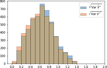
Distribution of $\sqrt{\operatorname*{Var}(V^*)}$ and $\sqrt{\operatorname*{Var}(\hat{V}^*)}$ in the $4021$ DGPs of our benchmark. Bins of 0.1 have been used.

If we subjectively consider that a standard deviation of less than 0.2 is a reasonable criterion for considering that the CATE problem has been transformed into a standard regression problem, we can see that this is not the case for most DGPs in our benchmark. There are only 254 DGPs such that $\sqrt{\operatorname*{Var}(V^*)}<0.2$ and 185 such that $\sqrt{\operatorname*{Var}(\hat{V}^*)}<0.2$. We can also observe that the median values for $\sqrt{\operatorname*{Var}(V^*)}$ and $\sqrt{\operatorname*{Var}(\hat{V}^*)}$ are respectively $0.622$ and $0.644$.

There are a few DGPs where $\sqrt{\operatorname*{Var}(V^*)}$ is close to its worst theoretical value. After a thorough examination, we noticed a pattern; these are causal-structure based DGPs where “opposing” causal populations (i.e. responders/anti-responders or survivors/doomed) are present in similar proportions and massively overlap. In general, in these DGPs, there are only 2 causal variables and opposing causal populations are normally distributed with means very close to each other.

In figure 2, we display the distribution of the RMSE of $\hat{V}^*$ (i.e. $\sqrt{\frac{1}{N}\sum(\hat{V}^*_i -\textcolor{green}{V^*_i})^2}$) throughout the benchmark.

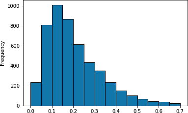
Distribution of the RMSE of $\hat{V}^*$ in the $4021$ DGPs of our benchmark.

We have used a unique approach to estimate $\hat{V}^*$ (a deep T-learner relying on binary cross entropy). We can see that for most of our DGPs, this results in an RMSE of less than 0.2 (median: 0.173), which can be considered acceptable. Also, we can observe that there are 443 DGPs with RMSE higher than 0.4, which indicates a poor estimation in our opinion. We have no a priori idea whether these are DGPs for which the chosen strategy was inappropriate or whether these DGPs are fundamentally intricate. For this, we computed the correlation between $\textcolor{green}{\sqrt{\operatorname*{Var}{V^*}}}$ (interpreted here as an index of the inherent intricacy of the DGP) and the RMSE of $\hat{V}^*$. We found a low correlation of 0.197, suggesting that the quality of the estimation of $\hat{V}^*$ is not strongly related to the intricacy of the DPG.

The quality of $\hat{V}^*$ as an estimator of the CATE thus changes a lot within the benchmark, and it is certainly interesting to try to understand how this impacts the performance of the models that rely on it.

6.2. $\hat{\mathcal{L}}^*$ vs. the AUUC

For each of our $4021$ DGPs and for each of the 11 model types (ECM is excluded), we have trained several models with different hyperparameters among which we want to select the best. In the end, we had $43830$ competitions to compare which of $\hat{\mathcal{L}}^*$ or the AUUC (henceforth refered to as $\mathcal{A}$) allows to make the better choice with respect to a ground-truth-based reference metric. Throughout all these competitions and for each reference metric, we count the number of times

$\hat{\mathcal{L}}^*$ selects a better model than $\mathcal{A}$,
$\mathcal{A}$ selects a better model than $\hat{\mathcal{L}}^*$,
$\hat{\mathcal{L}}^*$ and $\mathcal{A}$ selects models with an equal performance (which almost always means that they selected the same model).

reference metric	ex aequo	$\hat{\mathcal{L}}^*$ wins	$\mathcal{A}$ wins
RMSE	10671	28391	4768
$\textcolor{green}{\rho_{spearman}}$	10671	16722	16437
$\textcolor{green}{\tau_{kendall}}$	10671	16225	16934
$\textcolor{green}{\mathcal{G}_0'}$	10845	17141	15844

Table 2. Comparison of $\hat{\mathcal{L}}^*$ and the AUUC with respect to reference metrics

We can see in Table 2 that $\hat{\mathcal{L}}^*$ has an overwhelming superiority over $\mathcal{A}$ in terms of RMSE. However, this does not translate into a superiority in terms of $\textcolor{green}{\rho_{spearman}}$ $\ $and $\textcolor{green}{\tau_{kendall}}$. Our explanation is that the extent of the improvement of the individual prediction obtained through the use of $\hat{\mathcal{L}}^*$ is actually not big enough to lead to a significantly different ranking of samples as measured by $\textcolor{green}{\rho_{spearman}}$ or $\textcolor{green}{\tau_{kendall}}$. This actual extent can be seen in the next subsection that reports the models' performance.

As for $\textcolor{green}{\mathcal{G}_0'}$, we recall that this pragmatic metric, which is eventually the one of the most interest to the end user, measures only the ability of a model to predict correctly the sign of the uplift, as explained earlier. Improving the accuracy of individual prediction is certainly an advantage in that respect. However, the overall gain will be mainly due to samples with CATE around 0, which therefore contribute the least to the metric. Thus, selecting models according to $\hat{\mathcal{L}}^*$ leads only to a modest improvement over $\mathcal{A}$ in terms of $\textcolor{green}{\mathcal{G}_0'}$.

We also computed how many times each metric overstepped its boundaries, i.e. how many times the selected model had a better performance than the true model on the test set. We found that, out of the $43830$ generated models in this benchmark, we got:

$\mathcal{A}(\hat{\tau}) > \mathcal{A}(\textcolor{green}{\tau})$ : 5715 times.
$\hat{\mathcal{L}}^*(\hat{\tau}) < \hat{\mathcal{L}}^*(\textcolor{green}{\tau})$ : 840 times.
$\mathcal{A}(\hat{\tau}) > 1.01 \mathcal{A}(\textcolor{green}{\tau})$ : 3119 times.
$\hat{\mathcal{L}}^*(\hat{\tau}) < 0.99 \hat{\mathcal{L}}^*(\textcolor{green}{\tau})$ : 115 times.

From this point of view, $\hat{\mathcal{L}}^*$ seems also more reliable than the AUUC.

We conclude that the AUUC is slightly inferior to $\hat{\mathcal{L}}^*$ as a metric for the CATE task. However, we recall that, in our benchmark, we assume that $w$ is known, which is ideal for $\hat{\mathcal{L}}^*$ since it removes a source of noise and guarantees the AIPW pseudo-outcome to be consistent, whereas the AUUC needs not this extra information. Moreover, as practitioners, we are especially interested in $\textcolor{green}{\mathcal{G}_0'}$ and although $\hat{\mathcal{L}}^*$ has a small relative advantage in that respect, next section will show that very little is lost in terms of absolute value. Therefore, in the general case, we expect the AUUC to remain a safe choice whose practical advantages outweigh possible small losses of performance.

6.3. Models

In this section, we present the experimental results of all models. We decompose these results according to the many parameters of the DGPs in order to characterize their strengths and flaws. We also introduce some analysis of the local behaviour of each model. Since there are so many parameters, it is certainly possible to expand on these results beyond what we propose below.

Throughout this section, we highlight some observations that we found enlightening. We hope to stimulate a global scientific conversation about how these results should be further analysed. If it happens, we will include new elements in the next versions of this article.

6.3.1. General results

For every model type, we have selected two models: the best according to $\hat{\mathcal{L}}^*$ and the best according to $\mathcal{A}$. The average and the standard deviation of their scores on the whole benchmark with respect to our 4 ground-truth-based metrics are provided in table 3. We make the following observations:

model	RMSE	$\textcolor{green}{\rho_{spearman}}$	$\textcolor{green}{\tau_{kendall}}$	$\textcolor{green}{\mathcal{G}_0'}$
T-NN + $\hat{\mathcal{L}}^*$	17.1 (8.2)	84.3 (12.9)	71.1 (14.2)	5.5 (7.7)
T-NN + $\mathcal{A}$	17.2 (8.2)	84.3 (12.9)	71.0 (14.2)	5.5 (7.6)
SMITE* + $\hat{\mathcal{L}}^*$	16.5 (7.3)	84.2 (12.7)	70.7 (13.8)	5.6 (7.7)
DUR2 + $\hat{\mathcal{L}}^*$	16.1 (7.7)	83.1 (13.3)	69.3 (14.3)	5.7 (8.1)
DUR2 + $\mathcal{A}$	17.3 (7.5)	83.8 (13.2)	70.1 (14.3)	5.7 (8.1)
SMITE* + $\mathcal{A}$	16.8 (7.3)	84.0 (12.8)	70.5 (13.9)	5.8 (8.1)
SMITE + $\hat{\mathcal{L}}^*$	17.2 (7.5)	83.7 (13.0)	70.2 (14.1)	5.9 (8.1)
SMITE + $\mathcal{A}$	17.9 (7.5)	83.3 (13.4)	69.8 (14.3)	6.2 (8.7)
URF-V* + $\mathcal{A}$	23.0 (8.6)	83.9 (11.1)	69.1 (11.6)	6.6 (6.8)
URF-V* + $\hat{\mathcal{L}}^*$	23.0 (8.6)	83.9 (11.1)	69.1 (11.5)	6.6 (6.8)
URF-KL + $\mathcal{A}$	24.0 (8.7)	83.2 (11.6)	68.4 (12.0)	6.7 (7.0)
URF-KL + $\hat{\mathcal{L}}^*$	24.0 (8.7)	83.2 (11.6)	68.4 (12.1)	6.7 (6.9)
URF-ED + $\mathcal{A}$	23.2 (8.5)	83.4 (11.5)	68.5 (11.9)	6.8 (7.1)
URF-ED + $\hat{\mathcal{L}}^*$	23.2 (8.5)	83.4 (11.5)	68.5 (11.9)	6.8 (7.0)
URF-Chi + $\mathcal{A}$	26.5 (9.1)	82.2 (11.8)	67.2 (12.1)	7.1 (7.0)
URF-Chi + $\hat{\mathcal{L}}^*$	26.5 (9.1)	82.1 (11.9)	67.1 (12.2)	7.1 (7.0)
URF-CTS + $\hat{\mathcal{L}}^*$	25.5 (8.8)	82.8 (11.8)	67.8 (12.1)	7.4 (7.5)
URF-CTS + $\mathcal{A}$	25.5 (8.7)	82.8 (11.9)	67.8 (12.2)	7.4 (7.4)
T-RF + $\mathcal{A}$	25.7 (9.3)	79.4 (14.4)	64.1 (14.1)	9.2 (9.4)
T-RF + $\hat{\mathcal{L}}^*$	25.7 (9.3)	79.4 (14.5)	64.1 (14.2)	9.2 (9.4)
T-RL + $\hat{\mathcal{L}}^*$	30.3 (12.1)	70.0 (21.7)	55.0 (20.0)	16.2 (18.6)
T-RL + $\mathcal{A}$	30.3 (12.1)	70.0 (21.7)	55.0 (20.0)	16.2 (18.6)
ECM + $\mathcal{A}$	24.3 (15.0)	76.1 (21.0)	63.5 (22.1)	16.3 (19.9)
ECM + $\hat{\mathcal{L}}^*$	24.1 (14.8)	75.7 (21.5)	63.2 (22.4)	16.5 (20.3)

Table 3. The average and the standard deviation of their scores on the whole benchmark with respect to our 4 ground-truth-based metrics. Models are sorted according to $\textcolor{green}{\mathcal{G}_0'}$.

In terms of RMSE, neural nets clearly outperform the other models. For every model type, selecting the best model with $\hat{\mathcal{L}}^*$ leads to a better RMSE than selecting with the AUUC.
All metrics are topped in average by neural nets models selected with $\hat{\mathcal{L}}^*$. However, for metrics other than the RMSE, there is no clear difference between the performance of neural nets and random forests.
For some models like DUR$_{2}$, selecting with the AUUC leads to better performance with respect to true rank metrics.
As for random forests, the same hierarchy can be seen on every metric: URF-V$^* >$ URF-ED $>$ URF-KL $>$ URF-CTS $>$ URF-Chi
Perhaps disappointingly, the baseline neural net T-NN is a top contender. Even if it is beaten by DUR$_{2}$ and SMITE$^*$ on the RMSE as we hoped (since these latter models are trained to minimize $\hat{\mathcal{L}}^*$, an approximation of the MSE), but it still prevails on rank metrics and overall on $\textcolor{green}{\mathcal{G}_0'}$. The “naive” T-learner strategy is still strong.

Besides these average performances, we have also looked at how those models globally rank in the benchmark, i.e. how many times each model is first, second, etc. For each metric, we have a $24 \times 24$ table that we do not display here for space constraints. Considering the ranks do not alter the general impressions listed above but reveals an additional striking observation. We found, indeed, that the results of ECM are all-or-nothing; it actually comes first in 550 scenarios (with very few second places) and lies at the bottom most of the time. ECM is a parametric model and we have checked that it does indeed outperform the other models when it is correctly specified, i.e. when the causal populations have a Gaussian distribution. In addition, ECM is very sensitive: if we take a DGP which it comfortably tops and apply a few nonlinear bijective transformations of the covariates, its performance collapses and reaches the bottom. Therefore, as such, the ECM is unlikely to be reliable in a real word application, but this nevertheless suggests that it might be worthwhile to improve it by making it capable of handling other types of distributions. The authors have chosen to focus only on Gaussian distributions in the current implementation, but the principle of this algorithm could be adapted to many others.

6.3.2. DGP breakdown

Since there are $3900$ DGPs relying on the causal structure and $121$ on the response function, the results provided in table 3 are mostly characteristic of the causal-structure-based DGPs. In table 4 we highlight the performance on those response-function-based DGPs inspired from the literature.

model	RMSE	$\textcolor{green}{\rho_{spearman}}$	$\textcolor{green}{\tau_{kendall}}$	$\textcolor{green}{\mathcal{G}_0'}$
T-NN + $\hat{\mathcal{L}}^*$	10.4 (6.4)	84.9 (14.3)	72.4 (16.5)	7.4 (10.8)
T-NN + $\mathcal{A}$	10.7 (6.6)	84.5 (13.8)	71.9 (16.3)	7.4 (9.6)
DUR2 + $\hat{\mathcal{L}}^*$	11.6 (6.6)	81.8 (16.1)	67.8 (17.6)	8.5 (12.3)
SMITE* + $\hat{\mathcal{L}}^*$	11.8 (6.1)	83.7 (14.8)	70.6 (16.7)	7.5 (11.1)
SMITE* + $\mathcal{A}$	12.7 (6.4)	82.3 (16.0)	69.2 (17.6)	8.8 (13.5)
SMITE + $\hat{\mathcal{L}}^*$	13.6 (7.0)	81.1 (15.2)	67.7 (17.5)	9.6 (12.4)
DUR2 + $\mathcal{A}$	13.7 (6.5)	81.5 (16.7)	67.7 (18.3)	8.7 (11.7)
SMITE + $\mathcal{A}$	14.4 (7.3)	80.9 (15.8)	67.3 (17.8)	9.7 (12.6)
T-RL + $\hat{\mathcal{L}}^*$	17.7 (16.5)	86.1 (13.6)	73.2 (14.7)	8.3 (10.2)
T-RL + $\mathcal{A}$	17.7 (16.5)	86.1 (13.6)	73.2 (14.7)	8.3 (10.1)
URF-V* + $\mathcal{A}$	22.1 (13.2)	72.0 (19.6)	56.7 (17.9)	15.0 (15.9)
URF-V* + $\hat{\mathcal{L}}^*$	22.3 (13.1)	72.0 (19.4)	56.5 (17.7)	14.9 (15.4)
URF-ED + $\hat{\mathcal{L}}^*$	22.3 (13.1)	71.2 (20.1)	55.8 (18.2)	15.5 (15.9)
URF-ED + $\mathcal{A}$	22.4 (13.1)	71.2 (20.1)	55.9 (18.3)	15.6 (15.9)
URF-KL + $\hat{\mathcal{L}}^*$	22.7 (13.1)	71.5 (20.6)	56.5 (19.2)	15.4 (15.7)
URF-KL + $\mathcal{A}$	22.8 (13.2)	71.4 (20.5)	56.4 (19.1)	15.5 (16.0)
T-RF + $\mathcal{A}$	23.8 (13.5)	65.8 (19.9)	50.7 (17.9)	20.5 (17.8)
T-RF + $\hat{\mathcal{L}}^*$	23.8 (13.5)	65.8 (20.0)	50.7 (17.8)	20.7 (18.0)
URF-Chi + $\mathcal{A}$	23.8 (13.0)	71.3 (20.5)	56.4 (19.2)	15.5 (15.3)
URF-CTS + $\mathcal{A}$	23.9 (13.4)	71.1 (20.1)	55.8 (18.3)	15.8 (16.2)
URF-Chi + $\hat{\mathcal{L}}^*$	23.9 (13.1)	71.2 (20.8)	56.3 (19.4)	15.5 (15.7)
URF-CTS + $\hat{\mathcal{L}}^*$	23.9 (13.4)	71.1 (20.2)	55.7 (18.2)	16.0 (16.5)
ECM + $\hat{\mathcal{L}}^*$	24.0 (11.0)	72.1 (18.8)	57.5 (18.2)	19.8 (16.3)
ECM + $\mathcal{A}$	24.1 (11.1)	72.2 (18.6)	57.6 (18.1)	19.7 (15.9)

Table 4. Average performances and standard deviations on 121 response-based DGPs inspired from the literature.

We can see that the picture is different: in terms of RMSE, the absolute level of performance of neural nets is higher than on causal-structure-based DGPs and the two-classifier neural net prevails. Moreover, the two-classifier logistic regression also performs considerably better and is even the best performer with respect to $\textcolor{green}{\rho_{spearman}}$ and $\textcolor{green}{\tau_{kendall}}$. These facts suggest that those DGPs are indeed easier on average, with a structure most often appropriate to linear separation as performed by logistic regressions. As for ECM in the previous subsection, a closer examination shows that T-RL actually clearly dominates on scenarios from Tian (2012) [28] and Lo (2002) [29], while it performs poorly on the others. However, there are puzzling facts: the performance of random forests collapses in all respects and all models perform worse in terms of $\textcolor{green}{\mathcal{G}_0'}$.

It is then clear then that DGPs matter: differences in causal structures impact differently the models considered in this study and deeper analysis are required to understand the relationship between the characteristic of a DGP and the success or failure of a model.

Impact of DGP parameters on model's performance — Here we investigate the extent to which one-to-one modifications of the quantitative characteristics of the DGPs impact the performance of each model. These characteristics and their possible values in our benchmark are:

the number of samples $N$: 5000 or 20000;
the propensity $w$: 0.15, 0.3 or 0.5;
the number of nonlinear transformations of the data $nl$: from 0 to 15;
the number of causal features $c$ : 2, 5, 8;
the number of noncausal features $nc$ : 0, 2, 4, 8, 20, 32;
the variance of Gaussian distributions $\sigma$: 0.3, 1;
whether a linear transformation of the features has been applied at the end of response-based DGPs from the literature $l$.

Some parameters are not single quantitative indices: the quadruplet of causal population abundance $(\pi_R, \pi_S, \pi_D, \pi_A)$ and the mixture of distributions used to generate causal populations, which encompasses the nature of canonical distributions used (Gaussian or uniform) and the complexity of the mixture (up to 4 canonical distributions may have been used to generate a causal population). We chose to reduce these parameters to single indices (which obviously implies a loss information) in order to perform the same impact analysis as for the other parameters. Therefore, we chose to introduce the following new indices:

$\pi_R+\pi_A$, meant to somewhat capture the global strength of the CATE signal in a DGP (since the responders and anti-responders are the causal populations that drive its value away from 0). $\pi_R+\pi_A$ ranges from $0.2$ to $0.9$ in our benchmark.
The overall number of canonical distributions used in a DGP $n_{dist}$. It ranges from 4 to 11 in our benchmark.

We paired all DGPs that differ in only one of these characteristics and computed for each model type the variation in performance between all paired DGPs. The reference DGP is chosen as the one with the lowest value of the considered characteristic. There are 14854 of these unique pairs of DGPs. We focus on the RMSE as the reference metric of model performance. The average results are displayed in table 5.

	$N$	$nc$	$c$	$w$	$\sigma$	$nl$	$l$	$\pi_R+\pi_A$	$n_{dist}$
model	(1446)	(2145)	(920)	(2575)	(1972)	(1566)	(30)	(1379)	(3167)
DUR2	5.7	-2.7	-1.9	1.2	-2.6	-1.8	-1.8	-3.7	-1.1
T-NN	6.7	-3.0	-1.9	1.1	-3.1	-1.7	-3.2	-4.1	-0.8
SMITE*	5.6	-2.8	-2.5	1.1	-3.5	-1.5	-2.4	-3.5	-0.6
SMITE	5.9	-3.1	-2.9	1.2	-2.8	-1.4	-0.5	-3.6	-0.5
URF-V*	7.2	-1.8	-8.8	0.9	1.6	-2.1	-6.9	-2.5	-2.8
URF-CTS	6.4	-2.0	-8.7	0.7	2.1	-2.0	-6.3	-3.0	-2.9
URF-Chi	5.3	-2.1	-10.0	0.5	4.0	-1.5	-5.0	-2.4	-3.4
URF-ED	7.1	-1.8	-8.7	1.0	1.7	-2.1	-6.9	-2.5	-2.7
URF-KL	6.9	-2.0	-9.1	0.9	2.3	-1.9	-5.9	-2.4	-2.8
T-RF	8.2	-1.7	-10.1	1.7	2.3	-1.8	-6.5	-2.7	-2.5
T-RL	0.1	0.2	-6.4	0.2	2.6	-0.9	-0.1	-6.4	-3.5
ECM	1.2	-0.9	-1.9	2.0	-5.4	-7.1	-0.3	-9.7	-3.5

Table 5. Average variation of the RMSE of each model in % when increasing the parameters of the DGPs. For each parameter, the number of paired DGPs on which the average was computed is given in parentheses

We do not comment on the performance of ECM, T-RF or T-RL. Indeed, since their baseline performance is poor, we are not interested in their variations. We still report them for the sake of completeness.

We can see a number of expected trends and their actual extent:

All models benefit from larger data sets. For all models, increasing the size of the dataset from 5000 to 20000 samples leads to around 6% of improvement of the RMSE in average.
Increasing the number of variables in the problem decreases the performance of all models. In particular, increasing the number of causal variables has a more severe impact on random forests than on neural networks.
Increasing the propensity (which in our case means improving the test/control balance since we tested the values 0.15, 0.35 and 0.5) improves the performance of all models.
Performing non-linear transformations of the data impacts negatively the performance of all models.
Performing linear transformations of the data impacts negatively the performance of all models, with random forests being the most affected. Our interpretation is that before this transformation, there is a clear cut between causal and non-causal variables, which is naturally suited to a random forest's iterative single-variable split strategy. However, after the linear variable change, the causal signal spreads across all variables and becomes harder to map for a random forest.
Increasing $\pi_R + \pi_A$ has a negative impact on the performance of all models. Our interpretation is that a higher $\pi_R + \pi_A$ mostly leads to DGPs with a wider CATE range, which is likely to increase the estimation's errors of the model.
Neural models are more robust with respect to the inherent complexity of the distributions of causal populations as measured by $n_{dist}$.

Very interestingly, we also notice an unexpected behaviour: by increasing the variance of the Gaussian distributions used in our DGPs (which generates, on average, more overlapping of causal populations and increases the levels of $\operatorname*{Var}{V^*|x}$), the performance of neural nets decreases while that of random forests improves (even URF-V$^*$ which is based on $\hat{V}^*$).

6.3.3. Model performance as a function of the overlapping of causal populations

To better understand the latter observation, we plot the RMSE score made by each model on all the test sets of the benchmark in function of the local overlapping of causal populations as measured by $\eta$ (introduced in eq. \eqref{eta}). In other words, for each model we aggregate the $11542536$ predictions it made across all test sets of the benchmark and compute \begin{equation} \textcolor{green}{error(\eta)} = \sqrt{\mathbb{E}[(\hat{\tau}-\textcolor{green}{\tau})^2|\eta]}. \end{equation} Results are displayed in fig. 3.

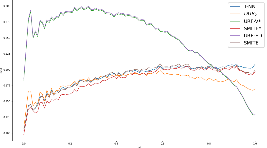
RMSE of models in function of $\eta$. Bins of 0.01 have been used.

This plot reveals peculiar local behaviours of models: random forests actually perform terribly in what are supposed to be “easy” regions, i.e. regions with low $\textcolor{green}{\eta}$, which mainly consist of one type of causal populations. This allows to make sense of the fact that increasing $\sigma$ in our benchmark led to better performances for random forests.

Within the neural networks category, SMITE$^*$ prevails when $\textcolor{green}{\eta}<0.53$ while DUR$_{2}$ prevails otherwise. Moreover, DUR$_{2}$ seems to improve as $\textcolor{green}{\eta}$ increases (i.e. the curve has a negative slope).

Obviously, describing the local behaviours of models according to a single index cannot capture the whole complexity of the situation. For instance, survivor-only regions and anti-responders-only regions both have $\eta=0$ and thus predictions on these regions have been merged and contribute to the same point of fig 3. However, the behaviour of some models in regions where $Y_i(1)=Y_i(0)$ might actually differ from regions where $Y_i(1) \ne Y_i(0)$.

When facing these curves, we obviously want to go further and try to investigate whether (and how) they are fundamentally related to the principle of each model or whether they are only induced by the peculiarities of our benchmark. We have indeed noticed a recent work [34] that addresses this issue in general and provides empirical evidence that a seemingly well-established models' hierarchy can be reversed by a few adjustments on the DGPs. If this is true and consistent, we hope at least that our introduction of $\eta$ will be helpful in exploring and understanding this dependency.

7. What is the best model?

As shown previously, T-NN, DUR$_{1}$ and SMITE$^*$ selected with $\hat{\mathcal{L}}^*$ already emerge as the best models in our benchmark although we certainly did not tap their full potential (we used the same architecture for all DGPs and optimized at most two hyperparameters). DUR$_{1}$ and SMITE$^*$ also depend more intimately on a quality estimation of $\hat{V}^*$, which could also be improved. If we had to pick only one model, it would be SMITE$^*$ since by combining $\hat{\mathcal{L}}^*$ and the binary cross entropy loss functions, it achieves a very close performance to the best for each reference metric while having a lower variance than other models, suggesting greater reliability.

However, we will try to go further by assuming that the local behaviours depicted in fig. 3 are indeed inherent to each model. If true, the best model would be actually a meta-model that picks the prediction of the most appropriate model depending on the local value of $\eta$. Since $\eta$ is not observable, it implies yet another preliminary training of an estimator $\hat{\eta}$, as for $V^*$. Since we can express both $\textcolor{green}{V^*}$ and $\textcolor{green}{\eta}$ (and the CATE...) in terms of $\textcolor{green}{\mu_1}$ and $\textcolor{green}{\mu_0}$ and since we have seen that T-learner strategy are very competitive, our practical recommendation would be then to estimate all of them at once by relying on the outputs $\hat{\mu}_1$ and $\hat{\mu}_0$ of a T-learner that ought to be trained as thoroughly as possible. Then $\hat{V}^*$ and $\hat{\eta}$ could be derived to train the other models and eventually build to the meta-model.

Our experimental results thus unexpectedly gives importance to the baseline T-learner strategy (which furthermore has the practical advantage not to rely on an estimation of $w$). This puts forth a question that has not been raised in our work: what is the best objective function to perform these two classifications? In this work we just used a standard binary crossentropy for each submodel of T-NN. Was there a better choice given the later use of $\hat{\mu}_1$ and $\hat{\mu}_0$ in $\hat{\mathcal{L}}^*$? We notice that if we rely on the same estimates of $\hat{\mu}_1$ and $\hat{\mu}_0$ to compute $\hat{\tau}$ and $\hat{V}^*$, we simply have

\begin{eqnarray*} \hat{\tau}(X_i)-\hat{V}_i &=& T_i\frac{\hat{\mu}_1(X_i) - Y_i}{w(x)} - (1-T_i)\frac{\hat{\mu}_0(X_i)-Y_i}{1-w(x)} \\ &=& \left\{ \begin{array}{ll} \frac{\hat{\mu}_1(X_i) - Y_i}{w(x)} & \mbox{\ if \ } T_i=1 \\ - \frac{\hat{\mu}_0(X_i)-Y_i}{1-w(x)} & \mbox{\ if \ } T_i=0 \end{array} \right. \\ \end{eqnarray*} and so $\hat{\mathcal{L}}^*$ simplifies to: \begin{equation} \hat{\mathcal{L}}^* = \sum\limits_{T_i=1} \frac{1}{w^2(x_i)}(\hat{\mu}_1(X_i) - Y_i)^2 + \sum\limits_{T_i=0} \frac{1}{(1-w(x_i))^2}(\hat{\mu}_0(X_i) - Y_i)^2 \label{T-opt} \end{equation}

It suggests that T-learners should just be trained by minimizing separately the MSE of Y on the test and control populations with inverse propensity weighting. This idea remains to be tested.

More tests are also required to substantiate the assumption of the meta-model, i.e that some models are fundamentally more appropriate on certain ranges of $\eta$ and that we can have an a priori idea of the boundaries of these ranges or dynamically find them.

8. Conclusion

In this article, we have proposed a new experimental set-up, performed experimental comparison of metrics, tested many diverse models and delved into their behaviour beyond mere global performance. We also proposed an alternative formulation of the AIPW pseudo-outcome and our new models. In conclusion, we share our humble opinion about what should be standardized, what should be deepened, and what remains to be done to further improve state of the art.

8.1. Take away

We believe that some of our approaches and results are worth standardizing in the future experimental developments of the topic:

In the case of binary treatment and outcome, benchmarks and axis of analysis of model predictions need to be standardised. Our contributions (causal-structure-based DGPs, analysis with DGP breakdown and with $\eta$) may constitute worthy elements for the subject's future.
At least when the propensity is known, $\hat{\mathcal{L}}^*$ is preferable to the AUUC to select models.
When synthetic data is used, it is interesting to assess model predictions with the ground truth (and do not only rely on the AUUC). The pragmatic $\textcolor{green}{\mathcal{G}_0'}$ metric is certainly a worthy index to look at in that respect.
The causal structure of the DGP is an interesting perspective to interpret results.
The T-learner is still a serious contender with appropriate means and should not be neglected.

8.2. Future works and open questions

In order to perfectly fulfill the original ambition of our work, several tasks and questions needs to be tackled:

Enriching the benchmark by expanding DGPs from the literature in the spirit of what we did (which was itself following the steps of [30]). Other real-world features could be added globally (i.e., categorical covariates, outliers, additional noise to simulate errors in covariate measurements...).
Expanding our comparison of metrics with new ones (see section 2.1).
Testing the objective function \ref{T-opt} for the T-learner.

We hope that this article will serve as a platform for a fruitful discussion that will result not only in the improvement of its content but also in the development of a shared vision of a CATE across all areas.

References

Donald B Rubin. “Estimating causal effects of treatments in randomized and nonrandomized studies.” (1974). Journal of educational Psychology, vol. 66, no. 5, p. 688.
Nicholas J Radcliffe. “Using control groups to target on predicted lift: Building and assessing uplift models” (2007). Direct Marketing Analytics Journal, vol. 1, no. 3, pp. 14–21.
Floris Devriendt, Jente Van Belle, Tias Guns and Wouter Verbeke. “Learning to rank for uplift modeling” (2020). IEEE Transactions on Knowledge and Data Engineering.
Artem Betlei, Eustache Diemert and Massih-Reza Amini, “Uplift modeling with generalization guarantees”. In Proceedings of the 27th ACM SIGKDD Conference on Knowledge Discovery & Data Mining, pp. 55–65 (2021).
Ikko Yamane, Florian Yger, Jamal Atif and Masashi Sugiyama. “Uplift modeling from separate labels” (2018). Advances in Neural Information Processing Systems, vol. 31.
Daniel G Horvitz and Donovan J Thompson. “A generalization of sampling without replacement from a finite universe” (1952). Journal of the American statistical Association, vol. 47, no. 260, pp. 663–685.
Susan Athey and Guido W Imbens. “Machine learning methods for estimating heterogeneous causal effects” (2015). stat, vol. 1050, no. 5, pp. 1–26.
James M Robins, Andrea Rotnitzky and Lue Ping Zhao. “Estimation of regression coefficients when some regressors are not always observed” (1994). Journal of the American statistical Association, vol. 89, no. 427, pp. 846–866.
Edward H Kennedy. “Optimal doubly robust estimation of heterogeneous causal effects” (2020). arXiv preprint arXiv:2004.14497.
Xinkun Nie and Stefan Wager. “Quasi-oracle estimation of heterogeneous treatment effects” (2017). arXiv preprint arXiv:1712.04912.
Peter M Robinson. “Root-N-consistent semiparametric regression” (1988). Econometrica: Journal of the Econometric Society.
Yan Zhao, Xiao Fang and David Simchi-Levi, “Uplift modeling with multiple treatments and general response types”. In Proceedings of the 2017 SIAM International Conference on Data Mining, pp. 588–596 (2017). SIAM
Sören R Künzel, Jasjeet S Sekhon, Peter J Bickel and Bin Yu. “Metalearners for estimating heterogeneous treatment effects using machine learning” (2019). Proceedings of the national academy of sciences, vol. 116, no. 10, pp. 4156–4165.
Maciej Jaskowski and Szymon Jaroszewicz, “Uplift modeling for clinical trial data”. In ICML Workshop on Clinical Data Analysis (2012).
Piotr Rzepakowski and Szymon Jaroszewicz, “Decision trees for uplift modeling”. In 2010 IEEE International Conference on Data Mining, pp. 441–450 (2010). IEEE
Michał Sołtys, Szymon Jaroszewicz and Piotr Rzepakowski. “Ensemble methods for uplift modeling” (2015). Data mining and knowledge discovery, vol. 29, no. 6, pp. 1531–1559.
Xiaogang Su, Joseph Kang, Juanjuan Fan, Richard A Levine and Xin Yan. “Facilitating score and causal inference trees for large observational studies” (2012). Journal of Machine Learning Research, vol. 13, p. 2955.
Susan Athey and Guido Imbens. “Recursive partitioning for heterogeneous causal effects” (2016). Proceedings of the National Academy of Sciences, vol. 113, no. 27, pp. 7353–7360.
Stefan Wager and Susan Athey. “Estimation and Inference of Heterogeneous Treatment Effects using Random Forests” (2015). arXiv preprint arXiv:1510.04342.
Leo Guelman, Montserrat Guillén and Ana María Pérez Marín. “Optimal personalized treatment rules for marketing interventions: A review of methods, a new proposal, and an insurance case study” (2014). UB Riskcenter Working Paper Series, 2014/06.
Victor Chernozhukov, Denis Chetverikov, Mert Demirer, Esther Duflo, Christian Hansen, Whitney Newey and James Robins, “Double/debiased machine learning for treatment and structural parameters” (2018).
Belbahri Mouloud, Gandouet Olivier and Kazma Ghaith. “Adapting Neural Networks for Uplift Models” (2020). arXiv preprint arXiv:2011.00041.
Christopher JC Burges. “From ranknet to lambdarank to lambdamart: An overview” (2010). Learning, vol. 11, no. 23-581, p. 81.
Céline Beji, Michaël Bon, Florian Yger and Jamal Atif. “Estimating Individual Treatment Effects through Causal Populations Identification” (2020). arXiv preprint arXiv:2004.05013.
Jennifer L Hill. “Bayesian nonparametric modeling for causal inference” (2011). Journal of Computational and Graphical Statistics, vol. 20, no. 1, pp. 217–240.
Jinsung Yoon, James Jordon and Mihaela Van Der Schaar, “GANITE: Estimation of individualized treatment effects using generative adversarial nets”. In International Conference on Learning Representations (2018).
Uri Shalit, Fredrik D Johansson and David Sontag, “Estimating individual treatment effect: generalization bounds and algorithms”. In International Conference on Machine Learning, pp. 3076–3085 (2017). PMLR
Lu Tian, Ash Alizadeh, Andrew Gentles and Robert Tibshirani. “A simple method for detecting interactions between a treatment and a large number of covariates” (2012). arXiv preprint arXiv:1212.2995.
Victor SY Lo. “The true lift model: a novel data mining approach to response modeling in database marketing” (2002). ACM SIGKDD Explorations Newsletter, vol. 4, no. 2, pp. 78–86.
Vincent Dorie, Jennifer Hill, Uri Shalit, Marc Scott, Dan Cervone et al.. “Automated versus do-it-yourself methods for causal inference: Lessons learned from a data analysis competition” (2019). Statistical Science, vol. 34, no. 1, pp. 43–68.
T Chan, Selim Esedoglu, Frederick Park and A Yip. “Total variation image restoration: Overview and recent developments” (2006). Handbook of mathematical models in computer vision.
Huigang Chen, Totte Harinen, Jeong-Yoon Lee, Mike Yung and Zhenyu Zhao. “Causalml: Python package for causal machine learning” (2020). arXiv preprint arXiv:2002.11631.
Nicholas J Radcliffe and Patrick D Surry. “Real-world uplift modelling with significance-based uplift trees” (2011). White Paper TR-2011-1, Stochastic Solutions.
Alicia Curth and Mihaela van der Schaar. “Doing great at estimating cate? on the neglected assumptions in benchmark comparisons of treatment effect estimators” (2021). arXiv preprint arXiv:2107.13346.
Antonio Gulli and Sujit Pal. “Deep learning with Keras”. Packt Publishing Ltd (2017).
F. Pedregosa, G. Varoquaux, A. Gramfort, V. Michel, B. Thirion, O. Grisel, M. Blondel, P. Prettenhofer, R. Weiss, V. Dubourg, J. Vanderplas, A. Passos, D. Cournapeau, M. Brucher, M. Perrot and E. Duchesnay. “Scikit-learn: Machine Learning in Python” (2011). Journal of Machine Learning Research, vol. 12, pp. 2825–2830.

Appendix

A. Ground truth of the DGPs of the literature

Here we present formulas for $\tau(x)$, $P(R|x)$ and $P(S|x)$ for different DGPs of the literature, with sketches of proof. $P(A|x)$ can be then calculated with $P(A|x) = P(R|x) - \tau(x)$ and $P(D|x)$ with $P(D|x) = 1 - P(R|x) - P(S|x) - P(A|x)$.

Notations — \begin{eqnarray*} \phi_\sigma(x) &=& (\sqrt{2\pi}\sigma)^{-1}\exp (\frac{-x^2}{\sigma}) \\ \Phi_\sigma(x) &=& \int_{-\infty}^x \phi_\sigma(y) dy \\ \eta(x) &=& \int_{-\infty}^x \Phi_\sigma(y) dy = x\Phi_\sigma(x) + \sigma^2\phi_\sigma(x) \mbox{\ (Proof: integration by parts)} \end{eqnarray*}

A.1. Response-based DG1 of type 1.

$Y_i = \mathbb{1}(f(x_i) + T_ig(x_i) + \epsilon_i >0)$ with $\epsilon_i \sim \mathcal{N}(0,\sigma)$ \begin{eqnarray*} \tau(x) &=& \Phi_\sigma(f(x)+g(x)) - \Phi_\sigma(f(x)) \\ p(R|x) &=& \left\{ \begin{array}{ll} \tau(x) & \mbox{\ if \ } g(x)>0 \\ 0 & \mbox{\ otherwise} \end{array} \right. \\ p(S|x) &=& \left\{ \begin{array}{ll} \Phi_\sigma(f(x)) & \mbox{\ if \ } g(x)>0 \\ \Phi_\sigma(f(x)+g(x)) & \mbox{\ otherwise} \end{array} \right. \end{eqnarray*}

A.2. Response-based DGP of type 2.

$Y_i = \mathbb{1}(\alpha_i + \epsilon_i >0)$ where $\alpha_i \sim U([a(x_i,T), b(x_i,T])$ and $a$ and $b$ are such that $a(x,T) < b(x,T) \forall x,T$. Notations : $a(x,0) = a_0$, $a(x,1) = a_1$, $b(x,0) = b_0$, $b(x,1)=b_1$, $I=(b_1-a_1)(b_0-a_0)$. We have $b_1>a_1$ and $b_0>a_0$. \begin{equation} \tau(x) = \frac{\eta(b_1) - \eta(a_1)}{b_1 - a_1} - \frac{\eta(b_0) - \eta(a_0)}{b_0 - a_0} \end{equation}

if $b_0 < a_1$: \begin{eqnarray*} p(R|x) &=& \tau(x) \\ p(S|x) &=& \frac{\eta(b_1) - \eta(a_1)}{b_1 - a_1} \end{eqnarray*}

if $b_1<a_0$: \begin{eqnarray*} p(R|x) &=& 0 \\ p(S|x) &=& \frac{\eta(b_0) - \eta(a_0)}{b_0 - a_0} \end{eqnarray*}

if $ b_1 > b_0 $ and $a_1 > a_0$: \begin{eqnarray*} I.p(R|x) &=& a_0(\eta(a_1) -\eta(b_1)) + b_1(\eta(a_0) - \eta(b_0)) + b_0\eta(b_1) - a_1\eta(a_0) \\ && - \sigma^2(\Phi(b_0)-\Phi(a_1)) \\ I.p(S|x) &=& b_1(\eta(b_0) - \eta(a_0)) + a_1\eta(a_0) - b_0\eta(a_1) + \sigma^2(\Phi(b_0)-\Phi(a_1)) \end{eqnarray*}

if $b_0>b_1$ and $a_0>a_1$: \begin{eqnarray*} I.p(R|x) &=& b_1\eta(a_0) - a_0\eta(b_1) - \sigma^2(\Phi(b_1) - \Phi(a_0)) \\ I.p(S|x) &=& b_0(\eta(b_1) - \eta(a_1)) + a_0\eta(a_1) - b_1\eta(a_0) + \sigma^2(\Phi(b_1)-\Phi(a_0)) \end{eqnarray*}

if $a_1<a_0$ and $b_1>b_0$: \begin{eqnarray*} I.p(R|x) &=& (b_0-a_0)(\eta(b_1)-\eta(a_1))-b_1(\eta(b_0)-\eta(a_0))-\sigma^2(\Phi(b_0)-\Phi(a_0)) \\ I.p(S|x) &=& b_1(\eta(b_0)-\eta(a_0))-(b_0-a_0)\eta(a_1)+\sigma^2(\Phi(b_0)-\Phi(a_0)) \end{eqnarray*}

if $a_1>a_0$ and $b_1<b_0$ \begin{eqnarray*} I.p(R|x) &=& (b_1-a_1)\eta(a_0) - a_0(\eta(b_1)-\eta(a_1))-\sigma^2(\Phi(b_1)-\Phi(a_1)) \\ I.p(S|x) &=& b_0(\eta(b_1)-\eta(a_1))-(b_1-a_1)\eta(a_0)+\sigma^2(\Phi(b_1)-\Phi(a_1)) \end{eqnarray*}

A.2.1. Proof for $\tau(x)$

With $\alpha_{ab} \sim U[a,b]$ and $\epsilon \sim \mathcal{N}(0,\sigma)$, the law $h_{ab\sigma}$ of $\alpha_{ab} + \epsilon$ is: \begin{eqnarray*} h_{ab\sigma}(z) &=& \int_{-\infty}^{+\infty} \frac{\mathbb{1}(a<y<b)}{b-a}\phi_\sigma(z-y)dy \\ &=&\frac{1}{b-a}\int_{a}^{b}\phi_\sigma(z-y)dy \\ &=&\frac{\Phi_\sigma(z-b) - \Phi_\sigma(z-a)}{b-a} \end{eqnarray*} Then we have \begin{equation*} p(Y=1|T=1,x) = \int_{0}^{+\infty}h_{a_1b_1\sigma}(y)dy = \frac{\eta(b_1)-\eta(a_1)}{b_1-a_1} \end{equation*} and similarly \begin{equation*} p(Y=1|T=0,x) = \frac{\eta(b_0)-\eta(a_0)}{b_0-a_0} \end{equation*}

A.2.2. Sketch of proof for $p(R|x)$

\begin{eqnarray*} p(R|x)&=& P(\alpha_{a_1b_1}+\epsilon>0) \ \& \ P(\alpha_{a_0b_0}+\epsilon<0) \\ &=& P( \alpha_{a_0b_0} < - \epsilon <\alpha_{a_1b_1} ) \\ &=& P( \alpha_{a_0b_0} < \epsilon <\alpha_{a_1b_1} ) \mbox{\ by symmetry}\\ &=& \int_{m,n} P(m<\epsilon<n) P(\alpha_{b_0a_0}=m,\alpha_{b_1a_1}=n ) \ dm \ dn \\ &=& \int_{m,n} P(m<\epsilon<n) P(\alpha_{b_0a_0}=m)P(\alpha_{b_1a_1}=n ) \ dm \ dn \\ &=& \int_{m=a_0}^{m=b_0}\int_{n=a_1}^{n=b_1} \frac{P(m<\epsilon<n)}{(b_1-a_1)(b_0-a_0)} \ dm \ dn \end{eqnarray*} Since $P(m<\epsilon<n) = 0$ if $m>n$ and $\Phi_\sigma(n) - \Phi_\sigma(m)$ otherwise, we end up with \begin{eqnarray*} I.p(R|x) &=& \int_D (\Phi_\sigma(n) - \Phi_\sigma(m)) \ dm \ dn \\ \mbox{\ with \ } D &=& \{(m,n), m \in[a_1,b_1], n \in[a_0,b_0], n>m\} \end{eqnarray*} Depending on the values of $a_0, a_1, b_0, a_1$, $D$ can be a triangle, a rectangle or a trapezium. One has to consider separately all cases and proceed with further decomposition of the integral.

A.2.3. Sketch of proof for $p(S|x)$

Similarly, we can show that \begin{equation} I.p(S|x) = \int_D \min(\Phi_\sigma(m) , \Phi_\sigma(n)) \ dm \ dn \end{equation} and again all cases have to be considered separately.

Response-based DGP 3. — $Y \sim \mathcal{B}(1, f(x,T))$ \begin{eqnarray*} \tau(x) &=& f(x,1)-f(x,0) \\ p(R|x) &=& f(x,1)(1-f(x,0)) \\ p(S|x) &=& f(x,1)f(x,0) \end{eqnarray*}

B. Additional technical details

B.1. Neural networks

Tools. — Neural networks were developed with the Keras library [35].

Parameter settings — . All neural networks use the following fixed settings:

optimizer: Adam
max number of epochs: 300
batch size: 256 for T-NN and 128 for all the others
the activation function of hidden layers is relu
neuron parameters are initialized using the RandomNormal procedure of TensorFlow

The optimal learning rate was looked for within the $[0.0001, 0.002]$ range.

The regularization coefficient of DUR$_{1}$ was looked for within the $[0,1]$ range

Early stop of training — We monitor the evolution of the loss on the validation set and interrupt the training process if the average of this loss over the last 5 epochs has not improved for 30 epochs.

B.2. Uplift random forests

We forked the library scikit-learn [36] and implemented uplift random forests using the same Cython optimization techniques already used for regular random forests. We achieved similar runtimes. We set the following ranges for random forests hyperparameters:

depth : $[7,23]$
number of trees : $[40,150]$
minimum number of samples per leaf : $100$

B.3. Early stop in 5-fold cross validation

When looking for the best hyperparameters of a model through 5-fold cross-validation, we try to detect an underperforming model early and save time by not training it on the 5 folds.

When optimizing a model with respect to $\hat{\mathcal{L}}^*$ or the AUUC, we keep track of the best current performance $K_{current\_best}$ that has been achieved for all sets of hyperparameters tested so far. When training a model with a new set of hyperparameters, after the 3rd and 4th fold, we compute its ongoing average performance $K_{on\ the\ fly}$ as well as its standard deviation $s_{on\ the\ fly}$ among those first 3 or 4 folds. If the metric considered is $\hat{\mathcal{L}}^*$ and if $K_{current\_best} < K_{on\ the\ fly} - s_{on\ the\ fly}$, then we consider that the current set of hyperparameters is unlikely to achieve a better performance than the current best and we do not train the model on the remaining folds. Similarly, if the metric is the AUUC, we check whether $K_{current\_best} > K_{on\ the\ fly} + s_{on\ the\ fly}$

Footnotes

1. We thank Christophe Renaudin from the Criteo R&D team for spectacularly speeding up the original implementation of this code.