Research article

A branch-and-bound algorithm for the prize-collecting single-machine scheduling problem with deadlines and total tardiness minimization

Version 1 Released on 15 April 2016 under Creative Commons Attribution 4.0 International License

Authors' affiliations

Dipartimento di Informatica - Università degli Studi di Milano
Dipartimento di Informatica - Università di Torino

Keywords

Abstract

We study a prize-collecting single-machine scheduling problem with hard deadlines, where the objective is to minimize the difference between the total tardiness and the total prize of the selected jobs. This problem is motivated by industrial applications, both as a stand-alone model and as a pricing subproblem in column generation algorithms for parallel machine scheduling problems. A pre-processing rule is devised to identify jobs that cannot belong to any optimal schedule. The resulting reduced problem is solved to optimality by a branch-and-bound algorithm and two integer linear programming (ILP) formulations. The algorithm and the formulations are experimentally compared on randomly generated benchmark instances.

Introduction

The single-machine scheduling problem has received growing attention in the scientific literature of the last decades, as shown by the reviews [1,2] and the many references therein. The problem with no release dates in which one wants to minimize the total tardiness ($1//\sum_j T_j$) was studied by Emmons [5]. Since it is weakly NP-hard, Lawler [3] provided decomposition rules to be exploited by dynamic programming. The problem with deadlines and total tardiness minimization ($1/\bar{d}_j/\sum_jT_j$) has received less attention: Tadei et al. [4] adapted the rules by Lawler [3] and Emmons [5] and proposed a B&B algorithm to solve the general case and derived conditions under which the problem can be solved in polynomial time. Analogous conditions were shown by Koulamas and Kyparisis [6] for the problem variant with release dates. In a more recent review Koulamas [2] stresses that the presence of deadlines makes the problem harder in the general case, although - at the best of our knowledge - it is still open whether such a problem is weakly or strongly NP-hard.

Oversubscribed scheduling is a research area of growing importance both for its many applications and for its intriguing combinatorial structure; it gives origin to prize-collecting scheduling problems or, equivalently, scheduling problems with rejection costs; the reader is referred to Shabtay et al. [7] for a recent survey on this topic. We are interested in the prize-collecting variant of the single-machine scheduling problem with deadlines and total tardiness minimization, where (at least a subset of) the jobs are not compulsory but their insertion in the schedule is awarded a prize in the objective function value. In particular we explicitly focus on oversubscribed scheduling, where the available processing time is insufficient for accommodating all jobs and one has to select a subset of jobs; the objective function to be maximized is the difference between the total tardiness and the prizes of the scheduled jobs. Several practical motivations exist for studying effective methods to solve prize-collecting scheduling problems: for example the heuristic algorithm presented by Wand and Tang [8] was motivated by applications in the iron and steel industry as well as in mechanical industry (e.g. cutting processes). Other applications are mentioned by Shabtay et al. [7], such as make-to-order production systems with limited production capacity and tight delivery requirements as well as scheduling with an outsourcing option. Oversubscribed scheduling problems also arise when machines represent highly valuable resources to be exploited at the maximum extent, as is the case with Earth observing satellites [16].

The same type of scheduling problem arises as a pricing sub-problem, when multi-machine scheduling problems are solved through column generation, where the prizes associated with the jobs are the optimal dual values provided by the linear relaxation of the master problem. However, such multi-machine scheduling problems have been so far investigated mainly for optimizing additive objective functions, such as the total (weighted) completion time of jobs or the (weighted) number of tardy jobs: see for example Chen and Powell [9] and van den Akker et al.[10]. The prize-collecting single-machine scheduling problems addressed in these cases were solved through pseudo-polynomial algorithms.

In this paper we address the prize-collecting single-machine scheduling problem with deadlines and total tardiness minimization. The initial motivation of our study was indeed the design and development of a column generation algorithm for a multi-machine scheduling problem to optimize the workforce management of computer analysts and code developers in a software house. The presence of constraints on deadlines makes our approach more general and better applicable: on one hand, pushing the deadlines far enough would reduce the problem to the easier total tardiness minimization scheduling problem, which can be seen as a special case of the problem with deadlines; on the other hand, hard deadlines can be quite important to model oversubscribed systems because in such a setting it may be worth scheduling jobs with large associated prizes even if their execution is scheduled largely after the due date; however, since scheduling problems are typically solved periodically at a tactical decision level, this phenomenon can repeat over and over, possibly causing negative effects (e.g. on relations with recurring customers). For this reason setting a maximum acceptable tardiness (i.e. a deadline) for each job may be necessary and therefore algorithms are needed that take this into account.

A prize-collecting single-machine scheduling problem with deadlines was addressed by Bilgintürk et al. [11] and by O\v{g}uz et al. [12]: however their model considers release dates and sequence-dependent setup times and it was solved with a linear integer model and several heuristic algorithms. Nobibon and Leus [13] addressed a single-machine scheduling problem with rejection costs and weighted total tardiness minimization but no deadlines; two linear integer programming models were formulated and two B&B algorithms were developed to solve the problem exactly.

In the following we formally define an ILP model of the problem (Section 2), we prove conditions to be tested to possibly detect dominated jobs that cannot belong to any optimal solution (Section 3), we illustrate a B&B algorithm that solves the problem exactly (Section 4) and we compare its results with those obtained by a general-purpose ILP solver (Section 5).

Two ILP models

From a given job set $J$ with cardinality $n$ some jobs must be selected for being processed on a machine. With each job $j \in J$ some data are associated, namely a processing time $p_j$, a due date $d_j$, a deadline $\bar{d}_j$ and a prize $\lambda_j$. The objective is to maximize the difference between the total prize of the selected jobs and their total tardiness, while respecting the deadlines. The tardiness $T_{j}$ of each job $j$ is the difference between the completion time of the job and its due date, if the former exceeds the latter; otherwise, it is zero. The cost for tardiness and the job prize are assumed to be converted in the same unit of measure, so that they can be subtracted from each other in the objective function. A given job subset $J_f \subseteq J$ includes mandatory jobs. The subset $J_f$ ensures that jobs that are crucial for particular reasons (e.g., have been already formally accepted or are requested by an important client) are performed even if they imply an overall loss ($T_j \geq \lambda_j$). The prize-collecting single-machine scheduling problem with total tardiness and hard deadlines can be indicated by $1/\bar{d}_j/\sum_jT_j+RC$ in symbolic scheduling language, where $RC$ represents the total rejection cost. Hereafter we present two integer linear programming formulation: the former is a model with positional variables, while the latter is a time-indexed formulation.

An ILP model with positional variables. This model is based on a formulation by Lasserre and Queyranne [14] for general scheduling problems. We elaborate on it to include the possibility of selecting some jobs. The model uses the following variables:

$x_{jh}\in\{0,1\}$ is equal to 1 if and only if job $j\in J$ is in position $h \in \{1,...,n\}$ in the schedule;
$y_h\in\{0,1\}$ is equal to 1 if and only if the schedule includes a job in position $h \in \{1,...,n\}$;
$C_h$ is the completion time of the job in position $h \in\{1,...,n\}$, if any;
$T_h\geq 0$ is the tardiness of the job in position $h \in\{1,...,n\}$, if any.

The ILP model is as follows. \begin{align} \min & \sum_{h \in \{1,...,n\}} \biggl(T_h - \sum_{j \in J} \lambda_j x_{jh}\biggr) & \label{Eq:Ppos:Obj}\\ & y_h = \sum_{j \in J} x_{jh} & h \in \{1,...,n\}, \tag{1b} \label{Eq:Ppos:YX}\\ & C_h \geq \sum_{h' \leq h} \sum_{j \in J} p_j x_{jh'} - M (1 - y_p) & h \in \{1,...,n\}, \tag{1c} \label{Eq:Cdef}\\ & T_h \geq C_h - \sum_{j \in J} d_j x_{jh} & h \in \{1,...,n\}, \tag{1d} \label{Eq:Tdef}\\ & T_h \leq \sum_{j \in J} (\bar{d}_j - d_j) x_{jh} & h \in \{1,...,n\}, \tag{1e} \label{Eq:dl}\\ & \sum_{h \in \{1,...,n\}} x_{jh} = 1 & j \in J_f, \tag{1f} \label{Eq:Jf}\\ & \sum_{h \in \{1,...,n\}} x_{jh} \leq 1 & j \in J\setminus J_f, \tag{1g} \label{Eq:onejob}\\ & T_h \geq 0 & h \in \{1,...,n-1\}, \tag{1h} \label{Eq:Tgeq0}\\ & y_h \geq y_{h+1} & h \in \{1,...,n-1\}. \tag{1i} \label{Eq:order} \end{align} Eq. \eqref{Eq:Ppos:Obj} defines the objective function as the difference between the total tardiness and the total prize. Eq. \eqref{Eq:Ppos:YX} relates the $x$ and $y$ variables. Eq. \eqref{Eq:Cdef} defines the completion time of the job in position $h$ as the sum of the processing times of all jobs before it; note that it is necessary to introduce a big-M term to allow for a zero completion time for positions where no job is processed. Eq. \eqref{Eq:Tdef} and \eqref{Eq:dl} define the tardiness variables and limit their values according to the deadlines. Eq. \eqref{Eq:Jf} and \eqref{Eq:onejob} ensure that each mandatory (respectively, facultative) job is processed exactly (respectively, at most) once, while Eq. \eqref{Eq:order} forces the occupied positions in the schedule to be contiguous. Note that when $T_j \geq \lambda_j$, the job is not worth processing and it can be discarded, unless $j \in J_f$. Therefore we can re-define the deadlines of non-mandatory jobs as \begin{equation} \bar{d}_j := \min\{\bar{d}_j, d_j+\lambda_j\}. \label{deadline} \end{equation} This can be done also for jobs with unspecified deadlines, if any exists. Tightening the deadlines can help to make a more effective use of the precedence rules that will be presented later on. Parameter $M$ needs to be larger than the largest deadline $\max_{j \in J}\{\bar{d}_j\}$. We observe that this formulation could be also adapted to the problem variation with weighted tardiness considered by Nobibon and Leus [13]; however this ILP formulation is different from theirs, since it does not require a variable $z_{ji}$ which takes value 1 if and only if job $j$ is selected and processed before job $i$. Avoiding these variables allows us to avoid a set of $\mathcal{O}(n^3)$ constraints into the model.

A time-indexed formulation. An alternative formulation, called the time-indexed (TI) formulation, was proposed by de Sousa and Wolsey [15]. Their idea is to discretise the time index $t \in \{1,...,t_{max}\}$ and to use a binary variable $z_{jt}$ that takes value 1 if and only if job $j \in J$ starts at $t \in \{1,...,t_{max}\}$. Note that if processing times, due dates and deadlines are not integer, they have to be re-scaled adopting a suitable elementary time unit. The value $t_{max}$ is to be set according to the largest deadline. The TI model also requires an additional parameter $c_{jt}$ which represents the cost of starting job $j \in J$ at time $t \in \{1,...,t_{max}\}$. \begin{align} \min & \sum_{j \in J} \sum_{t=1}^{\bar{d}_j-p_j+1} c_{jt} z_{jt} & \\ & \sum_{t=1}^{\bar{d}_j-p_j+1} z_{jt} \leq 1 & j \in J, \tag{3b} \\ & \sum_{j \in J} \sum_{s=t-p_j+1}^{t} z_{js} \leq 1 & t \in \{1,...,t_{max}\}, \tag{3c} \\ & z_{jt} = 0 & j \in J,\ \ t \in \{\bar{d}_j-p_j+2,t_{max}\}, \tag{3d} \\ & \sum_{t=1}^{\bar{d}_j-p_j+1} z_{jt} = 1, & j\in J_f. \tag{3e} \end{align} This model is equivalent to the second ILP model presented in Nobibon and Leus [13] with the addition of deadlines. The TI formulation is more general than the ILP model with positional variables, because it can account also for problems where the tardiness cost $c_{jt}$ of starting job $j \in J$ at time $t$ is not equal to $\max\{t+p_j-d_j,0\}$. A known disadvantage of the TI formulation is that the number of variables and constraints can grow very large if $t_{max}$ itself is large. However, its continuous relaxation generally gives better lower bounds [15]. We used both models as benchmarks to evaluate the branch-and-bound algorithm presented in the next sections. For this purpose we solved the two models with a state-of-the-art ILP solver. In the following we indicate them with $P_{\mathrm{pos}}$ and $P_{\mathrm{ti}}$ respectively.

Dominance and pre-processing

In this section we describe how jobs can be tested in order to detect whether some of them are dominated by others. This pre-processing test can even allow to discard some jobs from further consideration.

We define the following dominance property:

Property 3.1 Let us consider two distinct jobs $i,j \in J \setminus J_f$. If $p_i \leq p_j$, $d_i \geq d_j$, $\bar{d}_i \geq \bar{d}_j$, $\lambda_i \geq \lambda_j$ and at least one of the inequalities is strict, then job $i$ dominates job $j$, i.e. optimality is not lost by neglecting schedules that contain job $j$ and do not contain job $i$.

Proof. Assume an optimal schedule $S$ to contain job $j$ but not job $i$. Consider the schedule $S'$ obtained by replacing job $j$ by job $i$, with job $i$ starting in $S'$ at the same time as job $j$ starts in $S$ and leaving all starting times of the other jobs unchanged. $S'$ is feasible since $\bar{d}_i \geq \bar{d}_j$ and $p_i \leq p_j$ and then deadline constraints and no-overlap constraints are still satisfied in $S'$. The completion time of job $i$ in $S'$ is not larger than that of job $j$ in $S$, while all the other jobs are not affected. Since $d_i\geq d_j$, the total tardiness in $S'$ is not larger than the total tardiness in $S$. Since $\lambda_i \geq \lambda_j$, the total prize in $S'$ is not smaller than the total prize in $S$. Therefore $S'$ is also optimal. ∎

This property allows us to define a set of jobs that dominate each job $j \in J \setminus J_f$; we indicate such a set by $\Delta_j$. Consequently, some valid inequalities can be inserted in the ILP formulations illustrated in Section 2.

The following inequalities can be inserted in $P_{\mathrm{pos}}$: \begin{equation} \sum_{h \in \{1,...,n\}} x_{jh} \leq \sum_{h \in \{1,...,n\}} x_{ih}, \qquad j \in J \setminus J_f\ \ \ i \in \Delta_j. \tag{1.i} \label{valid_ILP} \end{equation} The following inequalities can be inserted in $P_{\mathrm{ti}}$: \begin{equation} \sum_{t \in \{1,\ldots,t_{max}\}} z_{jt} \leq \sum_{t \in \{1,\ldots,t_{max}\}} z_{it}, \qquad j \in J \setminus J_f\ \ \ i \in \Delta_j. \tag{2.f} \label{valid_TI-ILP} \end{equation} Once the dominating subsets $\Delta_j$ have been computed for each job $j$, we can exploit the following property:

Property 3.2 Consider a job $j \in J \setminus J_f$ with a subset of dominators $\Delta_j$ and consider any job $k \in \Delta_j \cup J_f \cup \{j\}$ such that $\bar{d}_k \geq \bar{d}_j$. If \begin{equation} \sum_{i \in \Delta_j \cup J_f \cup \{j\}: \bar{d}_i \leq \bar{d}_k} p_i > \bar{d}_k, \label{prop2} \end{equation} then job $j$ can be discarded without missing all optimal solutions.

Proof. When inequality (\ref{prop2}) is verified, not all jobs in $\Delta_j \cup J_f \cup \{j\}$ can be included in a feasible solution. Since the jobs in $J_f$ are mandatory and since each job $i \in \Delta_j$ dominates $j$, then, by property 3.1, job $j$ can be discarded in favor of jobs in $\Delta_j \cup J_f$ without losing all optimal solutions. ∎

Relying upon these two properties, it is possible to pre-process the instances in order to possibly tighten their formulation (by Property 3.1) or to reduce their size (by Property 3.2). The computational complexity of the pre-processing procedure is $O(n^2)$, because it requires to examine each pair of jobs. In Section 5. we report on the impact of dominance rules and pre-processing on the ILP formulations shown in Section 2. and on the B&B algorithm described in Section 4..

It is worth noting that this deadline-based pre-processing is generally applicable to single-machine scheduling problems with prizes (or rejection costs) and total tardiness minimization, even when deadlines are not specified as problem data. This is because they can be set as described in Section 2., equation (\ref{deadline}).

Branch-and-Bound

For the exact optimization of the prize-collecting single-machine scheduling problem with deadlines we designed a branch-and-bound algorithm that branches on the selectable jobs, either scheduling or rejecting each of them.

This is equivalent to branching on auxiliary binary variables $f_j = \sum_{p \in \{1...n\}} x_{jp}$ for each $j \in J\setminus J_f$ in formulation $P_{\mathrm{pos}}$; it is also equivalent to branching on auxiliary binary variables $f_j = \sum_{t\in\{1...t_{\max}\}}z_{jt}$ in formulation $P_{\mathrm{ti}}$.

For each sub-problem in the branch-and-bound algorithm, we compute a lower and an upper bound on its best solution. The computation of these bounds is illustrated in the remainder after a brief survey of the algorithm by Tadei et al. [4] which is used as a sub-routine within our branch-and-bound algorithm.

A subsidiary algorithm

The algorithm by Tadei et al. [4] is a depth-first-search branch-and-bound that computes the minimum total tardiness for a set $S=\{1,...,n\}$ of jobs to be scheduled on a single machine. An earliest ending time $e_j$ and a latest ending time $l_j$ are computed for each job $j \in S$. The algorithm makes intensive use of two properties:

Property 1: let $i,j \in S$ such that $i<j$,
(a) $i$ precedes $j$ if $d_i \leq \max\{e_j,d_j\}$ and $l_i \leq \bar{d}_j$.
(b) $i$ follows $j$ if $d_i > \max\{e_j,d_j\}$, $\bar{d}_i \geq l_j$ and $d_i + p_i > l_j$.
Property 2: if $\bar{d}_n \geq \sum_{i=1}^n p_i$ then job $n$ in position $k$ in the Early Due Date order can be optimally set in some position $r=k,...,n$ in the schedule. For any fixed $r$, the set of predecessors $B_n(r)$ and the set of successors $A_n(r)$ are given by
$B_n(r) = \{[1], [2], ... , [k-1], [k+1], ... , [r]\}$ and $A_n(r) = \{[r+1], ... , [n]\}$, where $[k]$ indicates the job in position $k$ in the Early Due Date Order.

These two rules are a generalization to the problem with deadlines of the rules proposed by Lawler [3] and Emmons [5] for the problem with no deadlines. Using the above properties allows to fix some jobs in the schedule so that the remaining jobs form blocks. These blocks are further restricted by a suitable branching mechanism.

Lower bounding

At each node of the branch-and-bound tree in our algorithm a lower bound is computed by independently optimizing the total tardiness and the total prize. The former must be minimized, the latter must be maximized, keeping into account the constraints coming from previous branchings. Let $J_{0} \subseteq J \setminus J_{f}$ and $J_{1} \supseteq J_{f}$ be the subsets of jobs for which $f_j$ has been fixed to $0$ and to $1$, respectively.

Since all jobs in $J_{1}$ must be scheduled, we compute the minimum total tardiness associated with these jobs, ignoring all the other jobs. This is done with the branch-and-bound algorithm of Tadei et al. [4]. The use of this subsidiary branch-and-bound algorithm to process a single sub-problem is justified by its velocity. However, when its running time becomes unacceptably large, the subsidiary branch-and-bound can be truncated, still returning a valid lower bound for the total tardiness.

To compute an upper bound on the total prize that can be achieved, we select the maximum prize subset of jobs (with respect to the prizes $\lambda_j$), complying with the deadlines. This corresponds to solving the following ILP problem:

\begin{align} \max\ & \sum_{j \in J} \lambda_j b_j & \label{Eq:LB:Obj} \\ & \sum_{j \in J: \bar{d}_j \leq \bar{d}_i} p_j b_j \leq \bar{d}_i & i \in J \tag{5b} \label{Eq:LB:Knapsack}\\ & b_j = 1 & j \in J_{1} \tag{5c} \label{Eq:LB:b1} \\ & b_j = 0 & j \in J_{0} \tag{5d} \label{Eq:LB:b0} \\ & b_j \in \{0,1\} & j \in J \tag{5e} \label{Eq:LB:Bin} \end{align} where $b_{j} = 1$ indicates that job $j$ belongs to the solution.

Since tardiness minimisation and prizes maximisation are done independently, the difference of the corresponding optimal values is a lower bound on the optimum value of the current sub-problem in the branch-and-bound algorithm.

Upper bounding

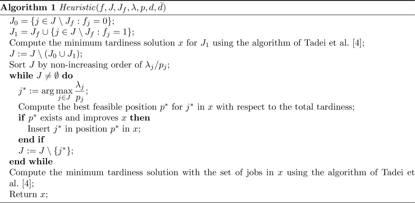
An upper bound is computed with a simple heuristic method that is run for each sub-problem of the branch-and-bound algorithm after the computation of the lower bound. It starts from the solution of the minimum tardiness sub-problem, which provides a feasible schedule for the jobs in $J_{1}$. The jobs from $J \setminus \left( J_{0} \cup J_{1} \right)$ are inserted in the current schedule, one by one, in non-increasing order of $\lambda_j/p_j$ (prize to processing time ratio), so as to improve the gained prize as much as possible while consuming the remaining working time as little as possible. Each new job is inserted in the position of the schedule where it provides the largest improvement to the objective value (i.e., where it yields the minimum increase in tardiness) and only if the insertion yields an improvement. When no more jobs can be profitably inserted, the current solution provides an upper bound. A pseudo-code is shown in Algorithm 1.

The branch-and-bound algorithm

A best incumbent upper bound is indicated by $UB^\ast$. It is initialized with the heuristic algorithm shown in Section 4.3. run on the whole instance with no fixed jobs.

Branching. We indicate by $0$-nodes and $1$-nodes the sub-problems of the branch-and-bound tree generated by setting a variable $f_j$ to $0$ and to $1$, respectively. We process each sub-problem $\nu$ (node, in the remainder) of the branch-and-bound tree as follows.

If $\nu$ is a $1$-node then solve the minimum tardiness sub-problem; otherwise keep the same optimal solution of the predecessor node. Let $T^*$ be the minimum tardiness.
If $\nu$ is a $0$-node, then solve the prize maximization sub-problem \eqref{Eq:LB}; otherwise keep the same optimal solution of the predecessor node. Let $P^*$ be the maximum prize.
Set the lower bound $LB^{\nu} := T^*-P^*$.
Compute an upper bound $UB^{\nu}$ with Algorithm 1.
If $UB^\nu < UB^{\ast}$, then update the best incumbent upper bound $UB^{\ast}$.
If $LB^{\nu} \geq UB^{\ast}$, then prune $\nu$.
If $\nu$ has not been pruned, then branch: select the job $j^* \in J \setminus \left( J_{0} \cup J_{1} \right)$ that belongs to the optimal solution of the prize maximization sub-problem \eqref{Eq:LB} and has the largest $\lambda_j/p_j$ ratio. Then generate two successor nodes by fixing $f_{j^*}$ either to 0 or to 1.

The branching rule aims at guaranteeing that the lower bound in the two successor nodes is larger than in the predecessor node. In fact, setting $f_{j^*} = 1$ makes an optimal solution of the minimum tardiness sub-problem infeasible, while fixing $f_{j^*} = 0$ makes an optimal solution of the maximum prize sub-problem infeasible.

Search strategy. The branch-and-bound tree is explored with best-first-search strategy: the next investigated sub-problem is the most promising one in the set of open sub-problems, that is the one with the smallest lower bound.

Computational experiments

In this section we report on the outcome of computational tests concerning the ILP formulations illustrated in Section 2. and the branch-and-bound algorithm described in Section 4.. The computations were performed on an eight-threads Intel(R) Core(TM) i7-3770 CPU with 3.40 GHz and 8 GB RAM. The branch-and-bound algorithm was coded in C++ and compiled with g++ 4.7.2, while the ILP formulations were solved with the C++ library of CPLEX 12.5.1.

Instances

We generated random instances as follows. We fixed the minimum and the maximum values of parameters $p$, $d$ and $\lambda$ and for each job we selected a random value in the allowed range, with a uniform probability distribution. The processing times and the due dates have minimum values at $p_{min} = 0.5$ and $d_{min} = 2$, while the maximum values are related to the total number of jobs, with the following combinations: $(|J|,p_{max},d_{max}) \in \{ (20,10,40),(40,15,80),(80,15,120),(120,20,200),(200,30,300) \}$. The rationale is to keep a direct correlation among the number of jobs, the maximum processing time and the maximum due date, in order to avoid the extreme opposite situations in which only very few jobs can be processed or all jobs can be easily processed respecting the due dates. The processing times were generated as rational numbers with a precision of $0.1$, while the due dates were generated as integer values. The prize of each job, $\lambda_{j}$, was extracted from the range $\left[ 1;10 \right]$ with uniform probability distribution and with a precision of $0.01$. The deadlines were derived from the due dates, generating $\bar{d}_j-d_j$ for each job $j$ as a random integer value with uniform probability distribution in $\left\{ 0,\ldots,10 \right\}$. For each of the triplets $(|J|,p_{max},d_{max})$ listed above, we generated five different random instances with an associated ID $i=1,\ldots,5$. Finally, for each instance we also generated a duplicate instance, where mandatory jobs are selected so that they require at least $25\%$ of the maximum available time. These jobs are chosen at random, but such that $J_f$ define a feasible set. Each of the resulting $50$ instances is represented by the quadruplet $(|J|,p_{max},d_{max},i)$, with an additional $f$ index attached for the instances with mandatory jobs.

Effectiveness of dominance rules and pre-processing

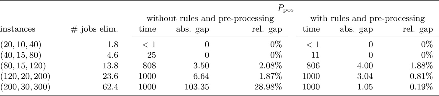
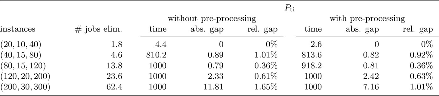
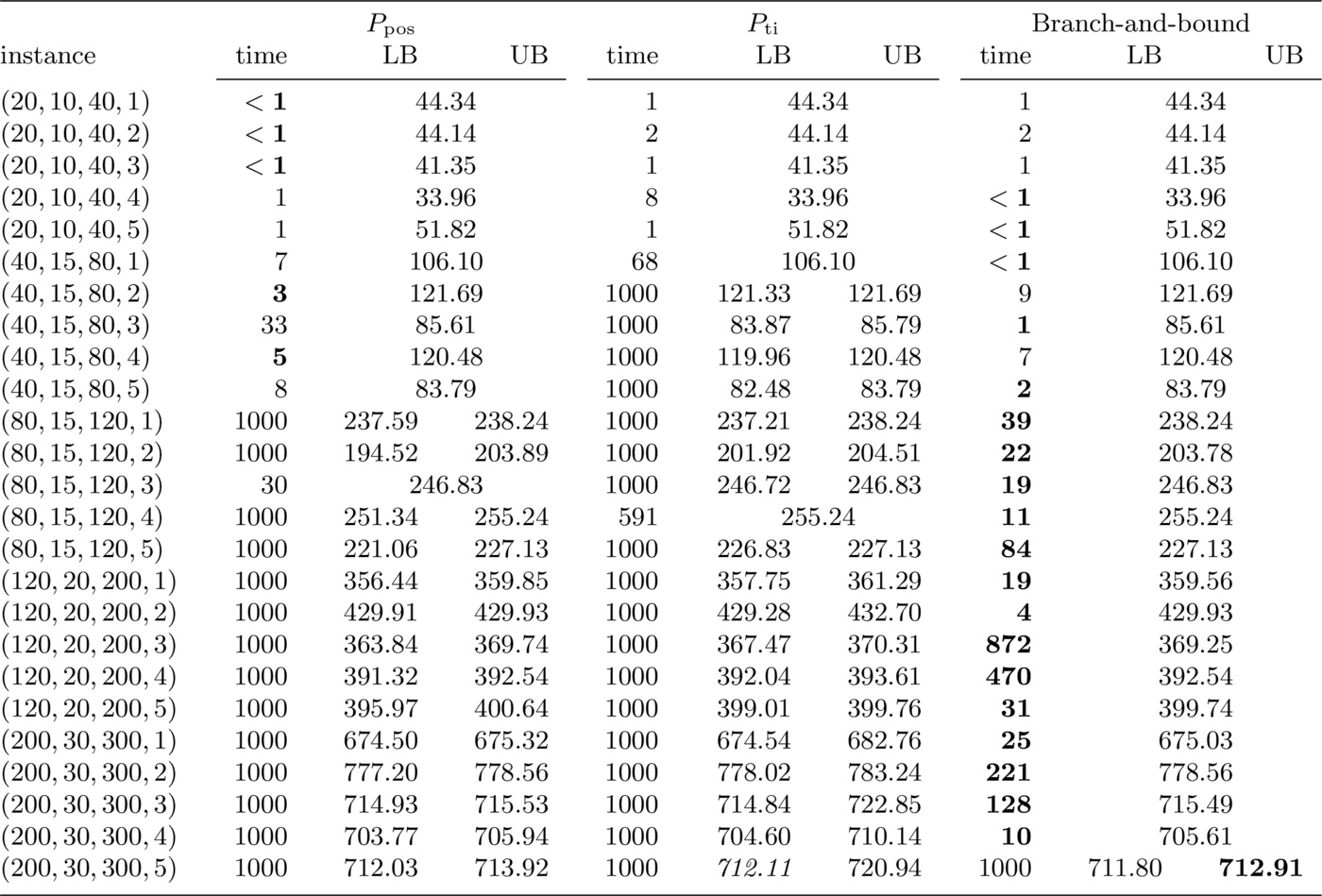
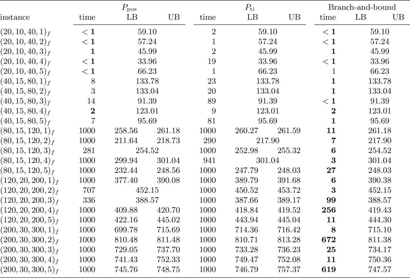
We designed a first set of computational tests to assess the effectiveness of dominance rules and pre-processing, as described in Section 3.. In Tables 1 to 3 we present the results obtained with Formulation $P_{\mathrm{pos}}$, Formulation $P_{\mathrm{ti}}$ and the branch-and-bound algorithm with and without dominance rules and pre-processing. Results have been obtained with a time-out of 1000 seconds. For each set of instances with given $|J|$, we display the average total running time in seconds and the average absolute and relative gap between the lower and the upper bounds. As stated in Section 2., we add the constant term $\sum_{j \in J} \lambda_j$ to the objective function of the ILP models, thus transforming our objective in a total tardiness penalty plus a total rejection cost, so that the objective function value (to be minimized) is always positive. The second column of each table indicates the average number of jobs eliminated by the pre-processing procedure: remarkably, the pre-processing eliminated up to one third of the jobs. In Section 3. we have also presented inequalities \eqref{valid_ILP} and \eqref{valid_TI-ILP} to tighten the two ILP formulations. Experimentally, we observed that the inclusion of inequalities \eqref{valid_TI-ILP} did not yield improvements when solving Formulation $P_{\mathrm{ti}}$; therefore these inequalities were not used in the next experiments. On the contrary, the results significantly improved when we included inequalities \eqref{valid_ILP} in Formulation $P_{\mathrm{pos}}$.

Table 1. Computational time (in seconds), absolute and relative gaps for Formulation $P_{\mathrm{pos}}$ without and with the use of valid inequalities and pre-processing, on the 25 instances with no mandatory jobs and a 1000 seconds time-out. Values are averaged on 5 instances of the same size.

Table 2. Computational time (in seconds), absolute and relative gaps for Formulation $P_{\mathrm{ti}}$ without and with the use pre-processing, on the 25 instances with no mandatory job and a 1000 seconds time-out. Values are averaged on 5 instances of the same size.

Table 3. Computational time (in seconds), absolute and relative gaps for the branch-and-bound algorithm without and with the use of pre-processing, on the 25 instances with no mandatory jobs and a 1000 seconds time-out. Values are averaged on 5 instances of the same size.

The results obtained with the two ILP formulations show similar improvements in computing time when the pre-processing was used. In particular, the results for the largest instances (200 jobs) were always better when pre-processing and dominance rules were used. This is particularly evident with Formulation $P_{\mathrm{pos}}$, where the primal-dual gap for instance $(200,30,300,3)$ was reduced by two orders of magnitude. The introduction of pre-processing and valid inequalities helped reduce the primal-dual gap mainly for the largest instances and it allowed closing the gap within the time-out for instance $(80,15,120,4)$ with Formulation $P_{\mathrm{ti}}$. Unfortunately, there was no beneficial impact on the quality of the lower bounds.

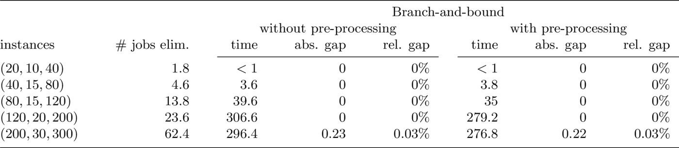
Using the branch-and-bound algorithm, the solution process of all instances with 80 jobs or more was enhanced by the pre-processing. The pre-processing reduced the computing time required by the branch-and-bound by only a handful of seconds on most instances; however, the gain was more significant when a large number of jobs was considered, as in instances $(200,30,300,2)$ and $(200,30,300,3)$.

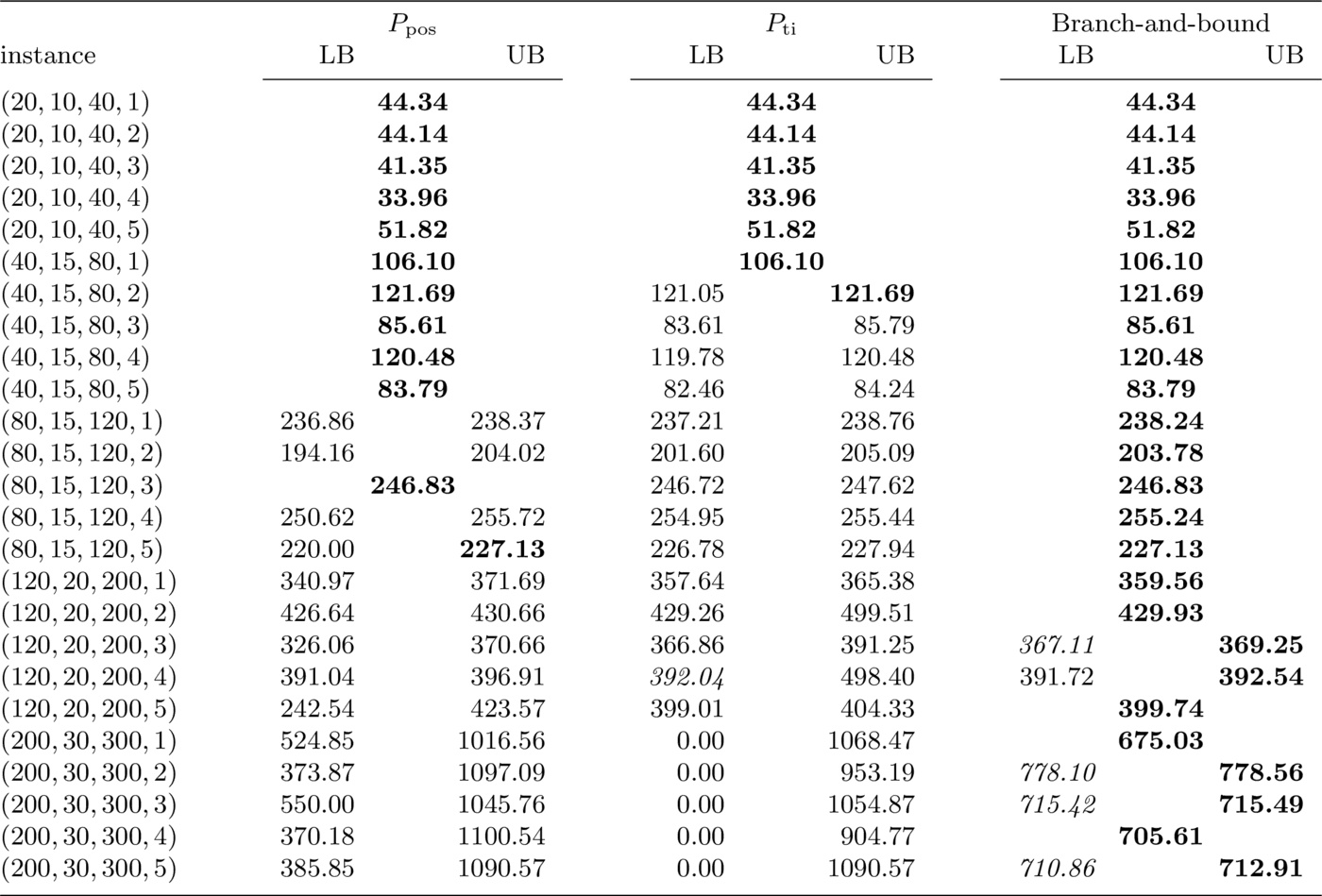
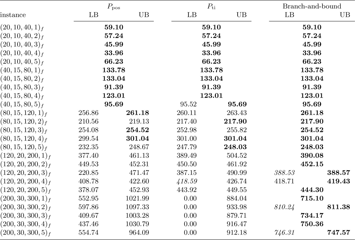
Comparison between methods

In this subsection we compare three methods for solving the prize-collecting single-machine scheduling problem with deadlines: the former two methods consist in solving the two ILP formulations shown in Section 2. with an ILP solver, while the third method is the branch-and-bound algorithm presented in Section 4., enhanced by the pre-processing and the dominance rules outlined in Section 3.. We also compare the results obtained with the three methods on the 25 instances with mandatory jobs: these results are reported in Table 5. We use bold fonts to put the best results in evidence. The computational results show poor performance of Formulation $P_{\mathrm{ti}}$, whose solution was generally slower than that of Formulation $P_{\mathrm{pos}}$ and the branch-and-bound algorithm. However, when other algorithms did not converge, formulation $P_{\mathrm{ti}}$ provided a better lower bound, in line with its reputation of yielding a tighter relaxation of the problem.

The branch-and-bound algorithm found proven optimal solutions within 1 000 seconds for all but one of 50 instances. Moreover, it provided the best results for all instances with 80 jobs or more (see Tables 1 to 3) and for all instances but one in Table 5. This is a remarkable feature of the branch-and-bound algorithm, since the other two methods could not close the gap within the time-out for instances with 80 jobs or more.

The branch-and-bound algorithm dominated the other two methods also in terms of bound tightness, with the only exception of the last instance with no mandatory jobs, where $P_{\mathrm{ti}}$ provided a better lower bound.

Table 4. Computational time (in seconds), lower and upper bounds for Formulation $P_{\mathrm{pos}}$, Formulation $P_{\mathrm{ti}}$ and the branch-and-bound algorithm (with pre-processing and dominance rules) with a timeout of $1\,000$ seconds. The smallest computing time within the time-out is displayed in bold font; if no algorithm converged, the best UB is displayed in bold font and the best LB in italic font.

Table 5. Computational time (in seconds), lower and upper bounds for Formulation $P_{\mathrm{pos}}$, Formulation $P_{\mathrm{ti}}$ and the branch-and-bound algorithm on the 25 instances with at least 25% of mandatory jobs, with a timeout at $1\,000$ seconds. The smallest computing time within the timeout is displayed in bold font; if no algorithm converged, the best UB is displayed in bold font and the best LB in italic font.

In order to assess the speed with which each algorithm was able to find good quality solutions, we also computed lower and upper bounds for each algorithm within a smaller time limit of 100 seconds. In these tests we focused on the values of the bounds, ignoring the computing time. The results are displayed in Tables 6 and 7. The best upper bounds are displayed in bold font, while the best lower bounds are displayed in italic. These results confirm the superiority of the branch-and-bound algorithm, which found the best upper bound for all 50 instances. We could also note that the lower and upper bound values for both ILP formulations on the largest instances sometimes drift quite far away from the optimum, thus providing unreliable estimations. On the contrary the branch-and-bound algorithm was able to provide the best LB more frequently than Formulation $P_{\mathrm{ti}}$ for the instances that remained unsolved after $100$ seconds. Even in the worst case, the primal-dual gap provided by the branch-and-bound algorithm was only a few units large. This suggests that, while the direct application of a state-of-the-art general-purpose solver does not provide a viable approach to the problem, the branch-and-bound algorithm can be used as a reliable heuristic in case of computing time shortage.

Table 6. Experimental results for the instances with no mandatory jobs, as in Tables 1 to 3, but with a time-out set at 100 seconds.

Table 7. Experimental results for the instances with mandatory jobs, as in Table 5, but with a time-out set at 100 seconds.

Conclusions

In this paper we have introduced the prize-collecting single-machine scheduling problem with total tardiness minimization and deadlines, a single machine scheduling problem that had not yet been studied before. The main motivation leading to our study came from an industrial multi-machine scheduling problem to be solved with column generation; however the specific prize-collecting scheduling problem is interesting in its own right for its intriguing combinatorial structure. We have presented a dominance rule between jobs as well as a rule to identify dominated jobs that can be deleted without losing optimal solutions. We have proposed two ILP formulations, that can be solved with general-purpose ILP solvers, as well as a specialized branch-and-bound algorithm where lower bounds are computed by exploiting an existing branch-and-bound algorithm for a simpler version of the problem. Computational results on randomly generated instances show that for 80 jobs or more the problem is difficult to solve for ILP solvers; this confirms the particular hardness of scheduling problems requiring total tardiness minimization. Our branch-and-bound algorithm was faster than a state-of-the-art ILP solver on almost all instances and provided small primal-dual gaps when the allotted computing time was made short enough to prevent the computation of optimal solutions.

Acknowledgments. The authors acknowledge the support of ACSU - Associazione Cremasca Studi Universitari to the OptLab, the Operations Research Laboratory of the University of Milan, where most part of this work was carried out. They also acknowledge the joint support of PA Digitale srl and Regione Lombardia through the programme “Dote Ricerca Applicata”.

References

- B. Chen, C.N. Potts and G.J. Woeginger, A Review of Machine Scheduling: Complexity, Algorithms and Approximability, Handbook of Combinatorial Optimization, D.-Z. Du and P.M. Pardalos (Eds), 1998 Kluwer Academic Publishers.
- C. Koulamas, The single-machine total tardiness scheduling problem: Review and extensions, European Journal of Operational Research 202 (2010) 1-7.
- E.L. Lawler, A pseudopolynomial algorithm for sequencing jobs to minimize total tardiness, Annals of Discrete Mathematics 1 (1977) 331–342.
- R. Tadei, A. Grosso and F. Della Croce, Finding the Pareto-optima for the total and maximum tardiness single machine problem, Discrete Applied Mathematics 124 (2002) 117–126.
- H. Emmons, One-machine sequencing to minimize certain functions of job tardiness, Operations Research 17 (1969) 701–715.
- C. Koulamas and G.J. Kyparisis, Single machine scheduling with release times, deadlines and tardiness objectives, European Journal of Operational Research 133 (2001) 447–453.
- D. Shabtay, N. Gaspar and M. Kaspi, A survey on offline scheduling with rejection, Journal of Scheduling 16 (2013) 3–28.
- X. Wang, L. Tang, A hybrid metaheuristic for the prize-collecting single machine scheduling problem with sequence-dependent setup times, Computers & Operations Research 37 (2010) 1624–1640.
- Z.L. Chen and W.B. Powell, Solving Parallel Machine Scheduling Problems by Column Generation, INFORMS Journal on Computing, 11:1 (1999) 78–94.
- J.M. van den Akker, J.A. Hoogeveen and S.L. van de Velde, Parallel Machine Scheduling by Column Generation, Operations Research 47:6 (1999) 862–872 .
- Z. Bilgintürk, C. O\v{g}uz and S. Salman, Order acceptance and scheduling decisions in make-to-order systems, 5th Multidisciplinary International Scheduling Conference: Theory and Applications (2007), Paris, France.
- C. O\v{g}uz, S. Salman and Z. Bilgintürk, Order acceptance and scheduling decisions in make-to-order systems, International Journal of Production Economics, 125:1 (2010) 200–211.
- F.T. Nobibon and R. Leus, Exact algorithms for a generalization of the order acceptance and scheduling problem in a single-machine environment, Computers and Operations Research 38:10 (2011) 367–378.
- J.-B. Lasserre , M. Queyranne, Generic scheduling polyhedral and a new mixed- integer formulation for single-machine scheduling, Proceedings of the 2nd Integer Programming and Combinatorial Optimization Conference (1992).
- J.P. de Sousa and L.A. Wolsey, A time-indexed formulation of non-preemptive single-machine scheduling problems, Mathematical Programming 54 (1992) 353–367.
- N. Bianchessi, G. Righini, Planning and scheduling algorithms for the COSMO-SkyMed constellation, Aerospace Science and Technology 12 (2008) 535–544.