Critical Casimir Force between Inhomogeneous Boundaries
Version 1 Released on 26 May 2015 under Creative Commons Attribution 4.0 International LicenseAuthors' affiliations
- Institut Jean Lamour, Physique de la Matière et des Matériaux (IJL/P2M). CNRS : UMR7198 - Université de Lorraine
- Laboratoire de Physique Théorique et Modèles Statistiques (LPTMS). CNRS : UMR8626 - Université Paris XI - Paris Sud
- Department of Physics, School of Science - MIT
- MultiScale Materials Science for Energy and Environment - Internation Joint Unit MIT/CNRS (UMI3466) *. Unregistered author (unverified)
Keywords
- Conformal field theory
- Critical behaviour in phase transitions
- Statistical physics
Abstract
To study the critical Casimir force between chemically structured boundaries immersed in a binary mixture at its demixing transition, we consider a strip of Ising spins subject to alternating fixed spin boundary conditions. The system exhibits a boundary induced phase transition as function of the relative amount of up and down boundary spins. This transition is associated with a sign change of the asymptotic force and a diverging correlation length that sets the scale for the crossover between different universal force amplitudes. Using conformal field theory and a mapping to Majorana fermions, we obtain the universal scaling function of this crossover, and the force at short distances.
Fluctuation-induced forces are generic to all situations where fluctuations of a medium or field are confined by boundaries. Examples include QED Casimir forces [1,2], van der Walls forces [3], and thermal Casimir forces in soft matter which are most pronounced near a critical point where correlation lengths are large [4,5]. The interaction is then referred to as critical Casimir force (CCF). Analogies and differences between these variants of the common underlying effect have been reviewed in Ref. [6].
Experimentally, CCFs can be observed indirectly in wetting films of critical fluids [7], as has been demonstrated close to the superfluid transition of ${}^4$He [8] and binary liquid mixtures [9]. More recently, the CCF between colloidal particles and a planar substrate has been measured directly in a critical binary liquid mixture [10,11]. Motivated by the possibility that the lipid mixtures composing biological membranes are poised at criticality [12,13], it has been also proposed that inhomogeneities on such membranes are subject to a CCF [14] which provides an example of a 2D realisation.
The amplitude of the CCF is in general a universal scaling function that is determined by the universality classes of the fluctuating medium [15]. It depends on macroscopic properties such as the surface distance, shape and boundary conditions of the surfaces but is independent of microscopic details of the system [5]. Controlling the sign of fluctuation forces (attractive or repulsive) is important to a myriad of applications in design and manipulation of micron scale devices. While for QED Casimir forces a generalized Earnshaw's theorem rules out the possibility of stable levitation (and consequently force reversals) in most cases [16], the sign of the CCF depends on the boundary conditions at the confinement. For classical binary mixtures, surfaces have a preference for one of the two components, corresponding to fixed spin boundary conditions ($+$ or $-$) in the corresponding Ising universality class. Depending on whether the conditions are like ($++$ or $--$) or unlike ($+-$ or $-+$) on two surfaces, the CCF between them is attractive or repulsive. So-called ordinary or free spin boundary conditions are difficult to realize experimentally but can emerge due to renormalization of inhomogeneous conditions as we shall show below [17]. Motivated by their potential relevance to nano-scale devices, fluctuation forces in the presence of geometrically or chemically structured surfaces have been at the focus recently. Sign changes of CCFs due to wedge like surface structures have been reported very recently [18]. Competing boundary conditions can give rise to interesting crossover effects with respect to strength and even sign of the forces. Here we consider such a situation for the Ising universality class in 2D. At criticality, this system can be described by conformal field theory (CFT) [19,20], and CCFs are related to the central charge of the CFT [21–23], and scaling dimensions of boundary operators [24].
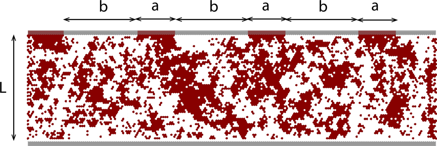 | Figure 1 Figure 1. Ising strip of width $L$ with alternating fixed spin boundary conditions on one side, with a typical spin configuation indicated by the shading. |
If the temperature is slightly different from $T_c$, the system is in the critical region, where the free energy density can be decomposed into non-singular (${\cal F}_{ns}$) and singular (${\cal F}_{s}$) contributions, \begin{equation} \label{eq:2} {\cal F}(t,L,\tau) = {\cal F}_{ns}(t,L,\tau)+ {\cal F}_s(t,L,\tau) \end{equation} that depend on the reduced temperature $t=T/T_c-1$, the width $L$, and a scaling variable $\tau=a/b-1$ that is specific to the alternating boundary conditions in Fig. 1. While the non-singular part is an analytic function of $t$ and $\tau$, the singular part is not. For homogeneous boundary conditions, $t$ is the only relevant scaling variable, and in the critical region the singular part of the free energy density is given by a universal scaling function $\vartheta$ that depends only on $L/\xi$ [15,5] where $\xi(t\to 0^\pm) = \xi_0^\pm |t|^{-\nu}$ is the bulk correlation length with amplitude $\xi_0^\pm$ and exponent $\nu=1$ for the Ising model. As we shall see below, the same renormalization-group (RG) concepts apply to a novel, boundary induced critical region that we identify for inhomogeneous boundary conditions around $a=b$. To focus on that region, we assume in the following that the system is at its bulk critical point, $t=0$. For large $L \gg a,b$ the singular part of the free energy density can be expressed in terms of a universal scaling function of the new correlation length $\xi_c(\tau)=(a+b)|\tau|^{-\nu_c}$, \begin{equation} \label{eq:3} {\cal F}_s(0,L,\tau) = \frac{1}{L} \vartheta[L/\xi_c(\tau)] \, . \end{equation} Below we shall determine $\vartheta$ and the exponent $\nu_c$.
BCC operators have been introduced in CFT to study systems with discontinuous boundary conditions [24]. When inserted on a boundary, these local operators interpolate between the different boundary conditions on either side of the insertion point. They are highest weight states of weight $h$ and all such states may be realized by an appropriate pair of boundary conditions. For the critical Ising model, the BCC operator that takes the boundary condition from $+$ spin to $-$ spin corresponds to the chiral part of the energy operator $\epsilon(z,\bar z)$. This can be understood easily in the representation of the Ising model in terms of a free Majorana fermion field $\psi(z)$ out of which the energy operator is composed, $\epsilon(z,\bar z)=i \psi(z)\bar\psi(\bar z)$ [25]: The Jordan-Wigner transformation shows that the fermion creation and annihilation operators flip locally the spin orientation.
Now the BCC operators permit us to relate the partition function of the strip with alternating boundary conditions to a correlator for the field $\psi(z)$ at positions where the boundary conditions change. On the upper complex plane, one has $\langle \psi(z)\psi(z')\rangle = 1/(z-z')$ which yields (after a conformal map) for the partition function of the strip the Pfaffian, \begin{equation} \label{eq:4} Z = Z_0 \langle \psi(w_1) \ldots \psi(w_{2N}) \rangle = Z_0 \text{Pf} (G) = Z_0 {\det}^{1/2} (G), \end{equation} with $G = [\langle \psi(w_i)\psi(w_j) \rangle]_{i,j=1,\ldots,2N}$, where we used the Wick theorem for fermions, $w_j$ are the positions of the $2N$ BCC operators on the upper edge of the strip, and $Z_0$ is the partition function of the homogenous system with $a=0$. Due to the symmetry under translations by $a+b$, the matrix $G$ is of block Toeplitz form, $G_{ij} = g_{i-j}$, with \begin{equation} \label{eq:5} g_j = \begin{pmatrix} g[j (a+b)] & g[j(a+b)-a] \\ g[j(a+b)+a] & g[j (a+b)] \end{pmatrix} \, , \end{equation} where $g(w)=\pi/[2L \sinh(\pi w / (2L)]$.
The free energy density can be expressed in the thermodynamic limit as \begin{equation} \label{eq:6} {\cal F} = -\frac{\pi}{48} \frac{1}{L} - \lim_{N\to\infty} \frac{1}{2N(a+b)} \log \det G \, . \end{equation} The Szegö-Widom (SW) theorem for block Toeplitz matrices states that the determinant can be expressed in terms of the matrix valued Fourier series $\varphi(\theta) = \sum_{k=-\infty}^\infty g_k e^{ik\theta}$ as [26] \begin{equation} \label{eq:7} \lim_{N\to \infty} \frac{1}{2N} \log \det G = \frac{1}{4\pi} \int_0^{2\pi} d\theta \log \det \varphi(\theta) \end{equation} where $\det$ acts now on a $2\times 2$ matrix. It turns out that this formula can be only applied for the case $a<b$. The reason for that is a subtle difference between the Toeplitz matrix $G$ and the corresponding circulant matrix $C$ that describes periodic boundary conditions along the strip. While for $a<b$ the spectra of $G$ and $C$ become equivalent for $N\to\infty$, for $a>b$ there exists a pair of eigenvalues of $GC^{-1}$ that tend to zero exponentially for $N\to\infty$, yielding an extra contribution $\delta$ that is determined by the decay of the Fourier integral \begin{equation} \label{eq:8} J=\frac{1}{2\pi} \int_0^{2\pi} d\theta e^{-i j \theta} \left[\varphi^{-1} (\theta)\right]_{11} \sim e^{-j \delta} \quad \text{for} \, j\to \infty \end{equation} and has to be subtracted from the r.h.s. of Eq. (\ref{eq:7}) for $a>b$. Here $\left[\varphi^{-1} (\theta)\right]_{11}$ denotes the $11$-element of the $2\times 2$ matrix $\varphi^{-1} (\theta)$. In the following we apply Eqs. (\ref{eq:7}) and (\ref{eq:8}) to compute the critical Casimir force in various scaling limits.
When $L\ll a,b$, the function $g(w)$ defined below Eq. (\ref{eq:5}) can be replaced by $g(w)=(\pi/L)e^{-\pi|w|/(2L)}$ which yields the exact determinant \begin{equation} \label{eq:9} \det \varphi(\theta) = \frac{\cos \theta -\cosh(\pi(a-b)/(2L))}{\cos \theta -\cosh(\pi(a+b)/(2L))} \, . \end{equation} For $a<b$, the SW theorem then yields $\frac{1}{2N}\log \det G = - (\pi a)/(2L)$. For $a>b$, this is also the correct result as it follows from subtracting the correction $\delta$ which follows from Eq. (\ref{eq:8}) and $J=e^{-\pi|a-b|j/(2L)}$ as $\delta=\pi(a-b)/(2L)$. It follows that the critical Casimir force for $L\ll a,b$ is \begin{equation} \label{eq:10} F = \frac{\pi}{48} \frac{23a-b}{a+b} \frac{1}{L^2} + \ldots \end{equation} It has an analytic amplitude that varies continously with $a/b$. This result is identical to an addition of the amplitudes from Eq. (\ref{eq:1}) for unlike and like boundary conditions, weighted by $a/(a+b)$ and $b/(a+b)$, according to their occurrence. Hence, additivity holds at short distances. This has been observed also for a 3D Ising model in the special case of boundaries with alternating stripes of equal width [17].
Next, we consider the case $L \gg a,b$. Using the Abel-Plana summation formula, it can be shown that in this limit the elements of the matrix \begin{equation} \label{eq:11} \varphi(\theta) = \frac{\pi}{L} \begin{pmatrix} i \gamma_1(\theta) & \gamma_2(\theta) \\ -\gamma^*_2(\theta) & i \gamma_1(\theta) \end{pmatrix} \end{equation} approach
where we have subtracted a $L$-independent contribution that does not change the force, and defined $\Gamma(\theta,\tau)=(2\hat\gamma_1+i(\hat\gamma_2-\hat\gamma^*_2)) /(|\hat\gamma_1|^2-|\hat\gamma_2|^2)$. In the evaluation of the integral, the correlation length $\xi_c(\tau)$ defined above Eq. (\ref{eq:3}) becomes important. The integrand is exponentially localized around $\theta=0, 2\pi$ over a small range $(a+b)/L$. Also, it can be shown that $\Gamma$ has the scaling property $\lim_{\tau\to 0} \Gamma( \tau^2/\zeta,\tau) = \Gamma_0(\zeta) = 1/(1+\pi^3\zeta/32)$ for any constant $\zeta$. Hence, in the critical region of small $\tau$, or $\xi_c(\tau) \gg a+b$, the proper scaling is obtained by setting $\zeta=(L\tau^2)/(a+b)=L/\xi_c$ (up to a numerical coefficient), showing that the exponent $\nu_c=2$. In the integral, $\Gamma(\theta,\tau)$ can be replaced by $\Gamma_0(\zeta)$ and one obtains after a simple integration the result for the universal scaling function of Eq. (\ref{eq:3}) when $a<b$ or $\tau<0$, \begin{equation} \label{eq:14} \vartheta_-(\zeta) = \frac{1}{4\pi} \text{Li}_2\left( \frac{2}{1+\pi^3 \zeta /32}-1\right) \end{equation} where $\text{Li}_2(x)=\sum_{k=1}^\infty x^k/k^2$ is a polylogarithm function. Outside the critical region $L\gg \xi_c$, one has $\vartheta_-(\zeta\to\infty) = -\pi/48$ so that the force is fully dominated by the boundary regions with like spins. On the contrary, for $L \ll \xi_c$, and hence $\tau\to 0^-$, the frustration between almost equal amounts of fixed $+$ and $-$ spins on the boundaries leads to a renormalization to effectively free boundary conditions with $\vartheta_-(\zeta\to 0) = \pi/24$. For $a>b$, the correction $\delta$ yields an extra contribution $\Delta\vartheta(\zeta)$ determined by \begin{equation} \label{eq:15} \Delta\vartheta(\zeta) \tan[\Delta\vartheta(\zeta)] = \frac{\pi^3}{32} \zeta \end{equation} so that the scaling function for $\tau>0$ is $\vartheta_+(\zeta) =\vartheta_-(\zeta) +\Delta\vartheta(\zeta)$. Since $\Delta\vartheta(\zeta\to 0)=0$, the scaling function is continuous around $\tau=0$. For $L \gg \xi_c$, however, $\Delta\vartheta(\zeta\to \infty)=\pi/2$ so that the system asymptotically realizes homogenous unlike boundary conditions with $\vartheta_+(\zeta\to \infty)=23\pi/48$.
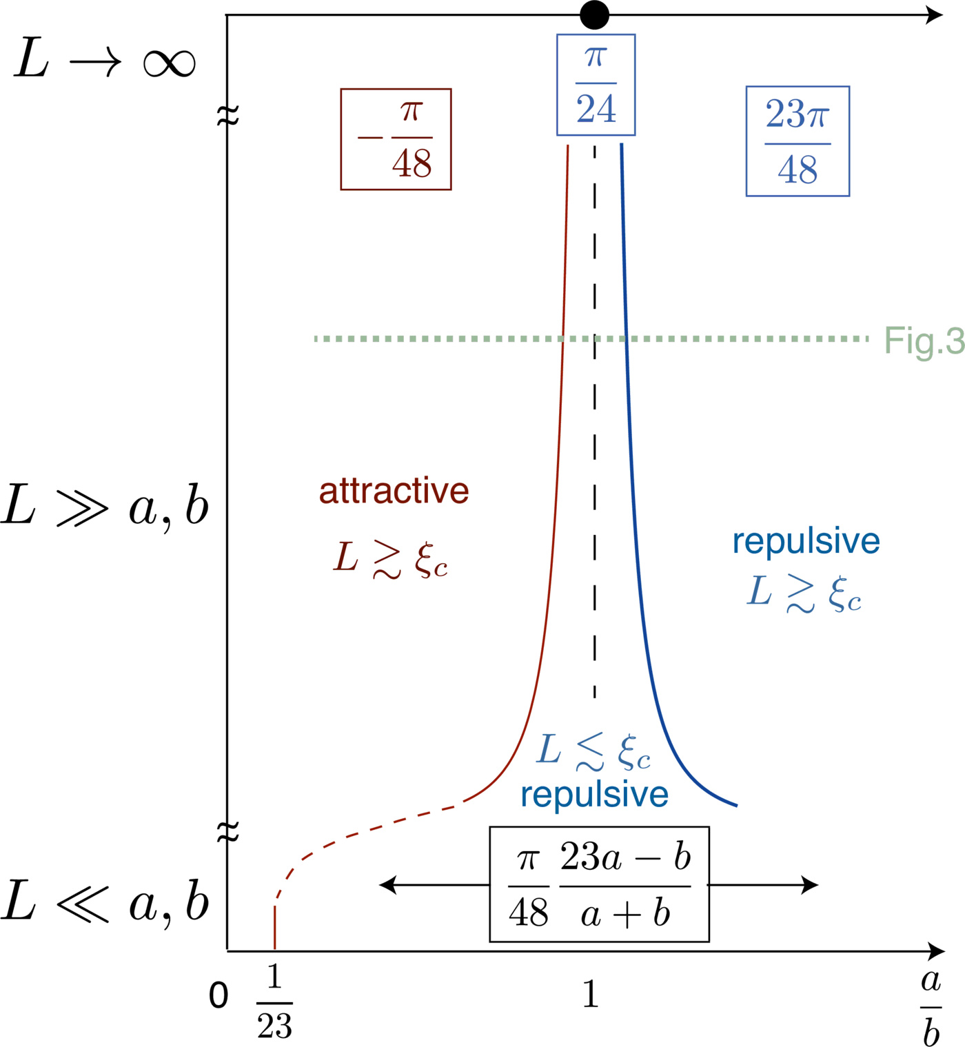 | Figure 2 Figure 2. Schematic overview of critical Casimir force amplitudes as function of the strip width $L$ and the ratio $a/b$. For $L\gg a,b$ the solid curves represent the diverging correlation length $\xi_c$. The horizontal dashed line indicates the cut along which the force amplitude is plotted in Fig. 3. Along the red curve the sign of the force changes whereas the blue curve indicates only a change between two universal (repulsive) limits. |
The dependence of the force $F$ on $|a-b|$ at fixed $L\gg a,b$ (see dashed horizontal line in Fig. 2) is determined by $F = -\partial {\cal F}/\partial L = \Theta(x_s) L^{-2}$ with a universal scaling function $\Theta$ of the scaling variable $x_s$ that is defined on both sides of the critical point by $x_s=\text{sign}(\tau)(L/\xi_c)^{1/2}\sim a-b$. This function is shown in Fig. 3 where we used the results for $\vartheta_\pm(L/\xi_c)$ of Eqs. (\ref{eq:14}), (\ref{eq:15}). In the critical region $|x_s| \ll 1$, one has the expansions \begin{equation} \label{eq:16} \Theta(x_s) = \left\{ \begin{array}{ll} \frac{\pi}{24} - \frac{\pi^2}{64} x_s^2 + \ldots & \text{for} x_s < 0 \\ \frac{\pi}{24} + \frac{\pi^{3/2}}{8\sqrt{2}} x_s + \ldots & \text{for} x_s > 0 \end{array}\right. \, , \end{equation} whereas for $L$ outside the critical region, $|x_s| \gg 1$, \begin{equation} \label{eq:17} \Theta(x_s) = \left\{ \! \begin{array}{ll} -\frac{\pi}{48} + \frac{32\log 2}{\pi^4} \frac{1}{x_s^{2}} + \ldots & \text{for} x_s < 0 \\ \frac{23\pi}{48} - \frac{32(\pi^2-\log 2)}{\pi^4} \frac{1}{x_s^{2}} + \ldots & \text{for} x_s > 0 \end{array}\right. . \end{equation} We see that $\Theta(x_s)$ is not analytic around $x_s=0$ and hence constitutes the singular part of the free energy density, see Eq. (\ref{eq:2}). This resembles the singular nature of scaling functions describing the bulk transition at $T=T_c$.
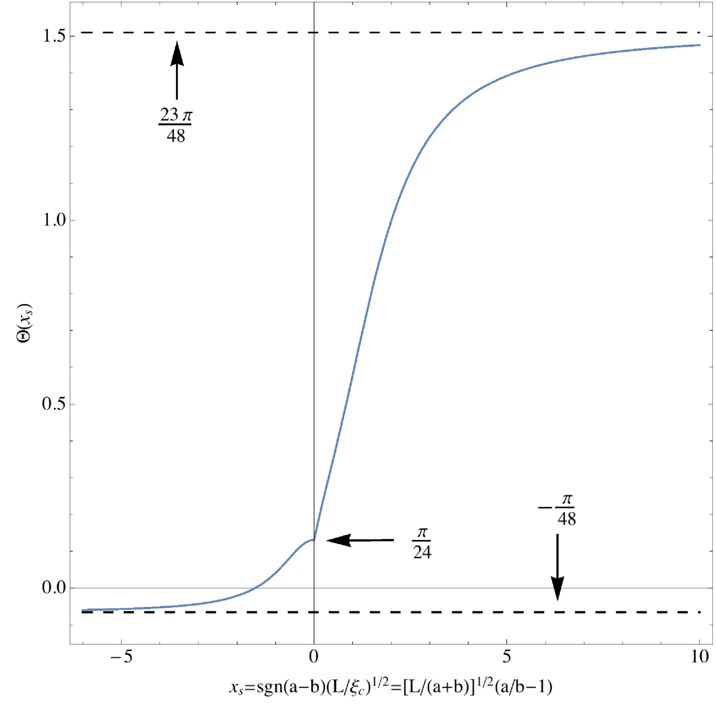 | Figure 3 Figure 3. Universal scaling function $\Theta(x_s)$ for the critical Casimir force as function of the scaling variable $x_s\sim a-b$. |
We thank M. Kardar for many fruitful discussions.
References
- H B G Casimir. Proc. K. Ned. Akad. Wet., 51:793, 1948.
- M Bordag, G L Klimchitskaya, U Mohideen, and V M Mostepanenko. Advances in the Casimir Effect. Oxford University Press, 2009.
- V. A. Parsegian. Van der Waals Forces. Cambridge University Press, 2005.
- P.-G. de Gennes and M. E. Fisher. C. R. Acad. Sci. Ser. B, 287:207, 1978.
- M Krech. The Casimir effect in Critical systems. World Scientific, 1994.
- A. Gambassi. J. Phys.: Conf. Ser., 161:012037, 2009.
- M. P. Nightingale and J. O. Indekeu. Phys. Rev. B, 32:3364, 1985.
- R. Garcia and M. H. W. Chan. Phys. Rev. Lett., 83:1187, 1999.
- R. Garcia and M. H. W. Chan. Phys. Rev. Lett., 88:086101, 2002.
- C. Hertlein, L. Helden, A. Gambassi, S. Dietrich, and C. Bechinger. Nature, 451:172, 2008.
- F. Soyka, O. Zvyagolskaya, C. Hertlein, L. Helden, and C. Bechinger. Phys. Rev. Lett., 101:208301, 2008.
- S. L. Veatch, O. Soubias, S. L. Keller, and K. Gawrisch. PNAS, 104:17650, 2007.
- T. Baumgart, A. T. Hammond, P. Sengupta, S. T. Hess, D. A. Holowka, B. A. Baird, and W. W. Webb. PNAS, 104:3165, 2007.
- B B Machta, S L Veatch, and J Sethna. Phys. Rev. Lett., 109:138101, 2012.
- Hans-Werner Diehl. Phase Transitions and Critical Phenomena, volume 10, page 75. Academic Press, London, 1986.
- S. J. Rahi, M. Kardar, and T. Emig. Phys. Rev. Lett., 105:070404, 2010.
- F. P. Toldin, M. Tröndle, and S. Dietrich. Phys. Rev. E, 88:052110, 2013.
- G. Bimonte, T. Emig, and M Kardar. Phys. Lett. B, 743:138, 2015.
- D. Friedan, Z. Qui, and S. Shenker. Phys. Rev. Lett., 52:1575, 1984.
- J. L. Cardy. In E. Brézin and J. Zinn-Justin, editors, Fields, Strings, and Critical Phenomena. Elsevier, New York, 1989.
- J Cardy. Nucl. Phys. B, 275:200, 1986.
- P Kleban and I Vassileva. J. Phys. A: Math. Gen., 24:3407, 1991.
- P Kleban and I Peschel. Z. Phys. B, 101:447, 1996.
- J. L. Cardy. Nucl. Phys. B, 324:581, 1989.
- P. di Francesco, P. Mathieu, and D. Sénéchal. Conformal Field Theory. Springer, 1997.
- Harold Widom. Adv. Math., 13:284, 1974.