Predicting global community properties from uncertain estimates of interaction strengths
Version 1 Released on 20 July 2017 under Creative Commons Attribution 4.0 International LicenseAuthors' affiliations
- Department of Physics, Chemistry and Biology (IFM), Institute of Technology - Linköping University
- Department of Ecology & Evolution, Division of Biological Sciences - University of Chicago *. Unregistered author (unverified)
Keywords
- Ecology
- Mathematical biology
- Qualitative properties of solutions
Abstract
The community matrix measures the direct effect of species on each other in an ecological community. It can be used to determine whether a system is stable (returns to equilibrium after small perturbations of the population abundances), reactive (perturbations are initially amplified before damping out), and to determine the response of any individual species to perturbations of environmental parameters. However, several studies show that small errors in estimating the entries of the community matrix translate into large errors in predicting individual species responses. Here we ask if there are properties of complex communities one can still predict using only a crude, order-of-magnitude estimate of the community matrix entries. Using empirical data, randomly generated community matrices, and those generated by the Allometric Trophic Network model, we show that the stability and reactivity properties of systems can be predicted with good accuracy. We also provide theoretical insight into when and why our crude approximations are expected to yield an accurate description of communities. Our results indicate that even rough estimates of interaction strengths can be useful for assessing global properties of large systems.
Introduction
Ecological communities can be modeled through a set of deterministic differential equations keeping track of population growth as a function of the (biotic and abiotic) environment. One central question in the study of communities is their stability [15]: when perturbing the population abundances slightly, does the community tend to return to its original state? This question naturally follows from the fact that, in nature, populations undergo constant perturbations, which they have to withstand to avoid extinction. Mathematically, a community equilibrium is locally stable if the Jacobian matrix, evaluated at that equilibrium, has eigenvalues with all negative real parts.
The Jacobian evaluated at an equilibrium point is called the community matrix [11], whose $(i,j)$th entry measures the change in the total population growth rate of species $i$ in response to a (small) change in species $j$'s abundance, in units of inverse time. This matrix has many useful properties in addition to determining local stability. For instance, a stable equilibrium is reactive [20] if perturbations, before damping, are initially amplified in a transient manner. Reactivity is measured by the leading eigenvalue of the Hermitian part of the community matrix, with positive values signaling reactive systems. In addition, the inverse community matrix can be used to determine the response of any species in the community to perturbations of the environment (i.e., not the abundances) via a community-wide sensitivity formula [12,6,29,18,2,4].
However, studies have revealed [29,30,8,21] that even small uncertainties in estimating the entries of the community matrix translate into large errors of prediction. The problem is that small perturbations to the matrix can have large effects on the inverse matrix, to the point where even the directionality of the species' responses to environmental perturbations are predicted erroneously. Since the eigenvalues of the inverse matrix are the inverses of the eigenvalues, we do not expect the inverse matrix to be ill-behaved as long as all eigenvalues are far from the origin of the complex plane. But problems arise when some eigenvalues are close to zero: then the slightest error in measurement may lead to qualitatively different outcomes. Suppose the leading eigenvalue of a community matrix is $(-0.01 \pm 0.02) / \text{year}$; its inverse is then either smaller than $-33.3 \; \text{years}$, or larger than $100 \; \text{years}$. A slight measurement error can make the difference in whether the inverse matrix is deemed to have a large negative or a large positive eigenvalue. We do not know for certain whether community matrices of large natural systems possess eigenvalues that are close to zero, but a heuristic argument can be made that this is indeed the case based on the shape of the species-abundance curve [17], which shows that rare species are always overrepresented in natural communities. Since even small perturbations of the abundances could knock such rare species to extinction, the system must lie close to a transcritical bifurcation, meaning that some eigenvalues are necessarily very close to zero.
In large systems, it is already logistically impossible to measure every pairwise interaction (a community of $100$ species with connectance $0.1$ has $1000$), let alone doing so with high accuracy. This fact, combined with the above argument, seems to imply the futility of relying on the “inverse problem” to obtain species' responses to environmental perturbations. What one can do, however—and this is the focus of our work—is to use imperfect information about the system to estimate properties which do not rely on inverting the community matrix, such as stability and reactivity. By avoiding the matrix inversion, small errors no longer translate into large ones, and so even crude estimates may provide useful information about a system.
Here we ask how well one can approximate the eigenvalue distribution of community matrices based on only an order-of-magnitude knowledge of interaction coefficients. Even though accurate measurement of all matrix entries is impossible, ecologists with extensive field experience can frequently rely on their intuition to classify interactions as “strong” or “weak”. We assume that the magnitude of the strongest interactions are known (reasoning that, since they are strong, they are the most likely to be noticed and possibly the easiest to measure), and coarse-grain each matrix entry into bins, based on their relative magnitudes in comparison to the strongest interactions. We show that the eigenvalue structure of complex community matrices can be captured well using this procedure, and therefore such qualitative information can be used to approximate system properties not relying on the inverse.
Below, after describing how we construct approximate matrices using imperfect data, we show how this procedure works on empirical datasets. We then apply the procedure to matrices that are randomly generated, as well as those generated by the Allometric Trophic Network model [7]. We then go on to give a theoretical justification to our method, building on the theory of random matrices [3] and pseudospectra [26]. We end by discussing the limitations of our approach and its relevance for the classic stability-complexity debate in community ecology.
Constructing approximate matrices
We are given a community matrix $A$, and we would like to know its eigenvalues, but information on $A$'s entries is limited. Quantitatively, we assume we know only the magnitudes of the largest positive and negative entry (denoted by $p$ and $n$, respectively), and the zero entries of $A$, i.e., we know which interactions are absent. Apart from this quantitative information, we assume a qualitative knowledge of all other matrix entries: based on expert opinion or other indirect information, we know whether a given entry is strong or weak compared to $n$ and $p$. Based on this, we assign numerical bins into which the entries of $A$ will be lumped. Let $B$ denote this binned approximation to $A$. We ask how well the spectrum of $B$ approximates that of $A$.
We thus need to specify a binning procedure. First, we choose a number of bins. We then assign numerical values to these bins. Finally, each entry of $B$ is set to the value of the bin closest to the value of the corresponding entry in $A$. For a given binning, we use the notation \[ (x_1, \; x_2, \; \ldots, \; x_k), \] meaning that the first bin goes from $x_1$ to halfway between $x_1$ and $x_2$, the second goes from halfway between $x_1$ and $x_2$ to halfway between $x_2$ and $x_3$, and so on, until the last bin going from halfway between $x_{k-1}$ and $x_k$ to $x_k$. As an example, consider the matrix \[ A = \begin{pmatrix} 7.8 & 6.7 & 3.7 & -1.2 \\ -7.5 & 2.6 & -7.4 & 0 \\ -10.0 & -6.9 & 0.4 & 5.8 \\ 0 & 0 & 10.0 & -8.7 \end{pmatrix} . \] Its strongest negative entry is $n = -10$; its strongest positive entry is $p = 10$. If we now decide to construct $B$ using three bins with values $(n, \; 0, \; p)$, we get \[ A = \begin{pmatrix} 7.8 & 6.7 & 3.7 & -1.2 \\ -7.5 & 2.6 & -7.4 & 0 \\ -10.0 & -6.9 & 0.4 & 5.8 \\ 0 & 0 & 10.0 & -8.7 \end{pmatrix} \quad \Rightarrow \quad B = \begin{pmatrix} 10 & 10 & 0 & 0 \\ -10 & 0 & -10 & 0 \\ -10 & -10 & 0 & 10 \\ 0 & 0 & 10 & -10 \end{pmatrix} . \] In principle, the choice for the number of bins and their values is arbitrary. Here we consider the following, more specific procedure. Let the number of bins be $k \ge 3$ an odd integer. Let us specify a binning resolution constant $b$ whose powers help define the bins; in effect, $b$ fixes the definition of an order of magnitude. The $k$ bins are then given by \[ (n, \; nb^{-1}, \; nb^{-2}, \; \ldots, \; nb^{-(k-1)/2}, \; 0, \; pb^{-(k-1)/2}, \; \ldots, \; pb^{-2}, \; pb^{-1}, p) . \] Using our previous example for $A$, we can bin $A$ with $k = 5$ and binning resolution $b = 10$. Since $n = -10$ and $p = 10$, the bins are $(-10, \; -1, \; 0, \; 1, \; 10)$: \[ A = \begin{pmatrix} 7.8 & 6.7 & 3.7 & -1.2 \\ -7.5 & 2.6 & -7.4 & 0 \\ -10.0 & -6.9 & 0.4 & 5.8 \\ 0 & 0 & 10.0 & -8.7 \end{pmatrix} \quad \Rightarrow \quad B = \begin{pmatrix} 10 & 10 & 1 & -1 \\ -10 & 1 & -10 & 0 \\ -10 & -10 & 0 & 10 \\ 0 & 0 & 10 & -10 \end{pmatrix} . \]
Our scheme for binning matrix entries involves exponentially shrinking bin sizes. Any number of other schemes may be implemented—e.g., linear binning, where adjacent bins are equally spaced. The reason for choosing the exponential scheme is that there is both theoretical [24] and empirical [28] evidence that the interaction strengths in large ecological networks follow a distribution close to lognormal. Therefore the exponential binning strategy is expected to yield better resolution of the underlying data than a linear one. This is not to say that different binning schemes are not better suited to different problems. However, regardless of the problem at hand, one should make sure that the procedure does not depend on the particular choice of units the matrix entries are expressed in, which means that the procedure should only be sensitive to the relative magnitudes of the matrix entries, not their actual numerical values which are unit-dependent. The exponential scheme obviously satisfies this requirement.
Exploratory analysis: some empirical datasets
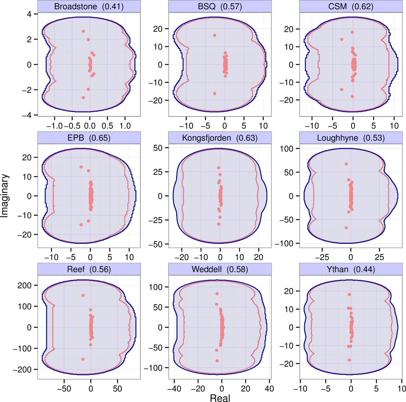
We show the eigenvalues (red dots) of community matrices from nine different empirical interaction webs in Fig. 1, parameterized using allometric scaling relationships [24]. These matrices were binned with $b=4$, $k=7$; the eigenvalues of the binned matrices (blue circles) are also shown. The number of species in each web is indicated in the panel titles. To interpret the eigenvalue distributions correctly, note the scale discrepancy between the real and imaginary axes.
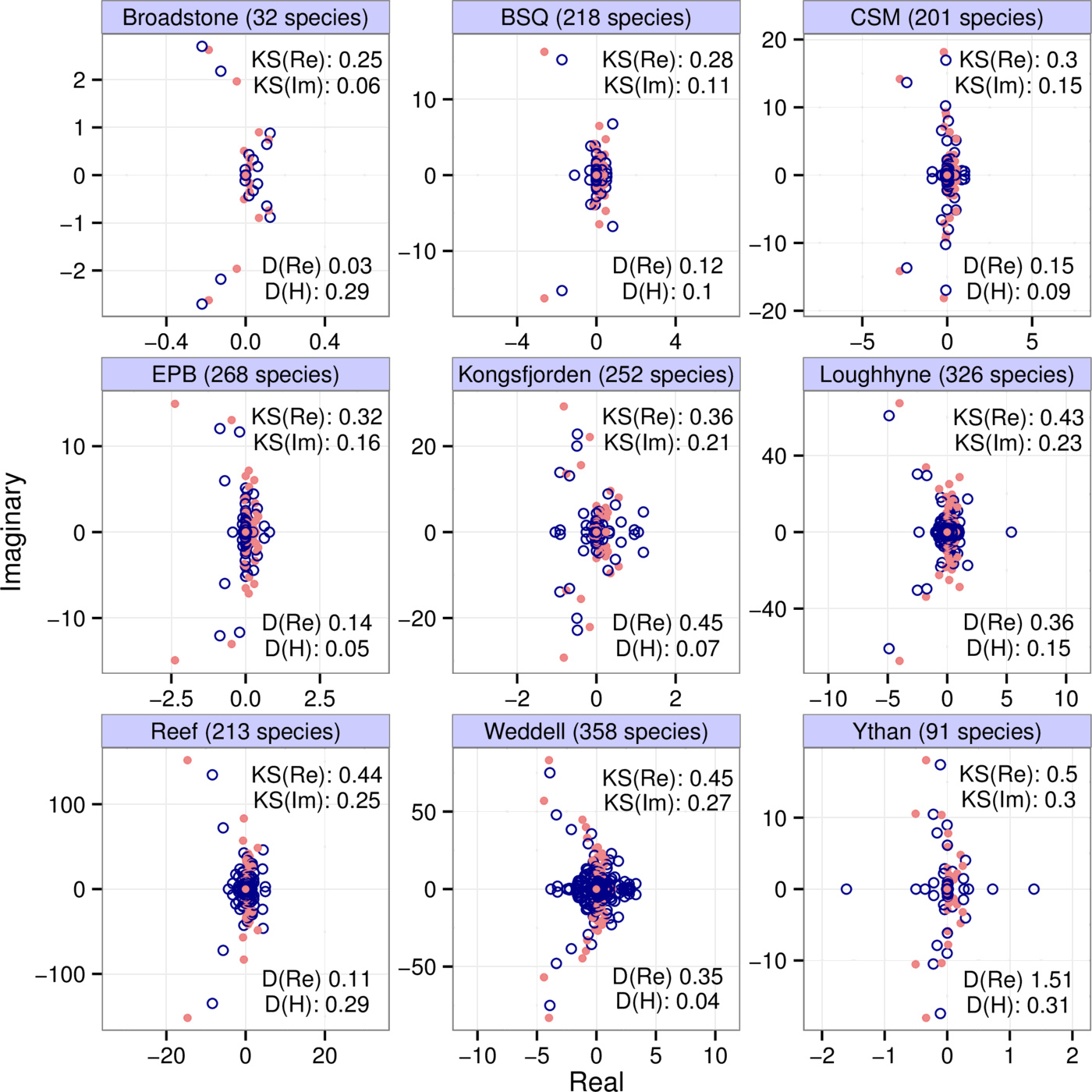
From the point of view of local stability, the leading eigenvalue (that with the largest real part) is of crucial importance: the sign of the real part of this eigenvalue determines whether the system is stable (negative) or unstable (positive). We consider the difference between the leading eigenvalues of the binned and original matrices to see how well it is captured. However, the raw difference itself is not informative, since the numerical value of this eigenvalue difference simply depends on the choice of units we measure the matrix entries in. A better question is how well the leading eigenvalue of the original matrix is approximated compared to the total spread of the eigenvalues; that is, can we say that the leading eigenvalue of the binned matrix is close to that of the original one, compared to the total range of the real parts of all the eigenvalues of the original matrix? These values are included in the panels under “D(Re)”. We can see that, for the datasets presented, the binning approximation always errs on the conservative side, overestimating the actual leading eigenvalue. This conservatism is due to the fact that our method of matrix binning include both largest entries of the matrices as bins, and also the zero bin. The binning procedure will lump several entries into these extreme bin values. Therefore the variance of the entries of the binned matrix will in general exceed that of the original matrix, which leads to a higher variance in the eigenvalue distribution as well.1
Note that none of the matrices in Fig. 1 are stable. This is because the empirical studies which they are based on only document trophic links, with no data on self-interactions. Due to this lack of information, we set all diagonal entries to zero. However, since the sum of the diagonal entries of a matrix is also the sum of its eigenvalues, such matrices cannot be stable. Their instability is therefore likely an artifact of our ignorance rather than an actual phenomenon. However, since we are interested in the ability of binned matrices to approximate spectra (whether they are stable or not), this lack of information is not a problem for us here.
Just as with stability, we can also examine reactivity, measured by the leading eigenvalue of $A$'s Hermitian part $H(A) = (A + A^{\top})/2$; $A^{\top}$ is the transpose of $A$. We therefore calculate $H(A)$ and $H(B)$, and ask how well the leading eigenvalue of the latter approximates that of the former in comparison with the total spread of the eigenvalues of $H(A)$. The results, for the empirical webs of Fig. 1, are shown under “D(H)”.
Let us highlight some of the general conclusions from these motivating examples. First, the eigenvalue distributions of the original and binned matrices roughly overlap: their means and variances are very similar in both the real and imaginary directions. Second, some of the finer structure of the eigenvalues distributions is also captured: more eigenvalues near the origin, and a few ones protruding in arcs toward the left half plane. Third, despite these features, the match between the actual and predicted values for stability and reactivity is not always very close—cautioning that the approximation could fail to capture specific numerical estimates for these properties. The method therefore reveals the general features of the system, and gives a rough idea of the quantitative details.
Randomly generated interaction matrices
Here we test the binning procedure on randomly generated interaction matrices. For each matrix we first fixed the number of species $S$ and the connectance $C$. We then generated two uniform random numbers between 0 and 1 to determine the types of all nonzero interactions. The first number is the fraction of trophic interactions, the second the fraction of mutualistic ones out of those that were nontrophic (the rest of the interactions were designated competitive). For each of the three interaction types there was an associated probability distribution from which the matrix entries pertaining to the interaction type in question were drawn. The procedure for generating the probability distribution was the same in all cases: first, the shape of the probability distribution was determined: either lognormal or Gamma. (We did this to check the robustness of our results to the choice of the underlying distribution. The results are indeed robust; see Supporting Information, Figs. S23-S26). Second, the mean and standard deviation of the distribution were uniformly sampled: for the mean, from $[0.1, \; 10]$, and for the standard deviation, from $[1, \; 10]$. For the trophic interactions, a random conversion efficiency was uniformly sampled from $[0.05, \; 0.2]$ to take into account the limited energy flow between trophic levels. To set the diagonal of the matrix, we sampled each diagonal entry from either a lognormal or a Gamma distribution, times $-1$ to keep the diagonal entries negative. The mean and standard deviation of the distribution were randomly drawn as in the offdiagonal case. See the Supporting Information for a more detailed breakdown of our method for generating these matrices.
We repeated the parameterization for four different values of the species richness $S$ ($50$, $100$, $250$, and $500$) and of the connectance $C$ ($0.1$, $0.25$, $0.5$, and $1$), in all possible combinations. Then, $300$ replicates of all cases were generated. All resulting matrices were binned, based on all possible combinations of the following three variables. First, the number of bins was chosen to be either $3$, $5$, $7$, or $9$. Second, the binning resolution was set to $2$, $4$, $6$, $10$, and $14$. Third, we took into account the effect of accidentally misclassifying matrix entries. In empirical situations, it seems likely that strong interactions may accidentally be deemed weak (or vice versa), given the insufficient, qualitative information one uses to generate approximate matrices. We therefore explored what happens when we deliberately misclassify some fraction of the matrix entries. In doing so, we assumed that zero interaction strengths do not get misclassified (absent interactions cannot ever be observed, and so will not be accidentally classified as present), and that the bin category of a nonzero interaction can only move up or down one bin (a strong interaction may be misclassified as weak, but not as zero). We used three rates of misclassification: $0\%$, $10\%$, and $20\%$. Our results were not strongly affected by misclassification (Supporting Information, Figs. S1-S5). Here in the main text we always show results with a $10\%$ misclassification rate.
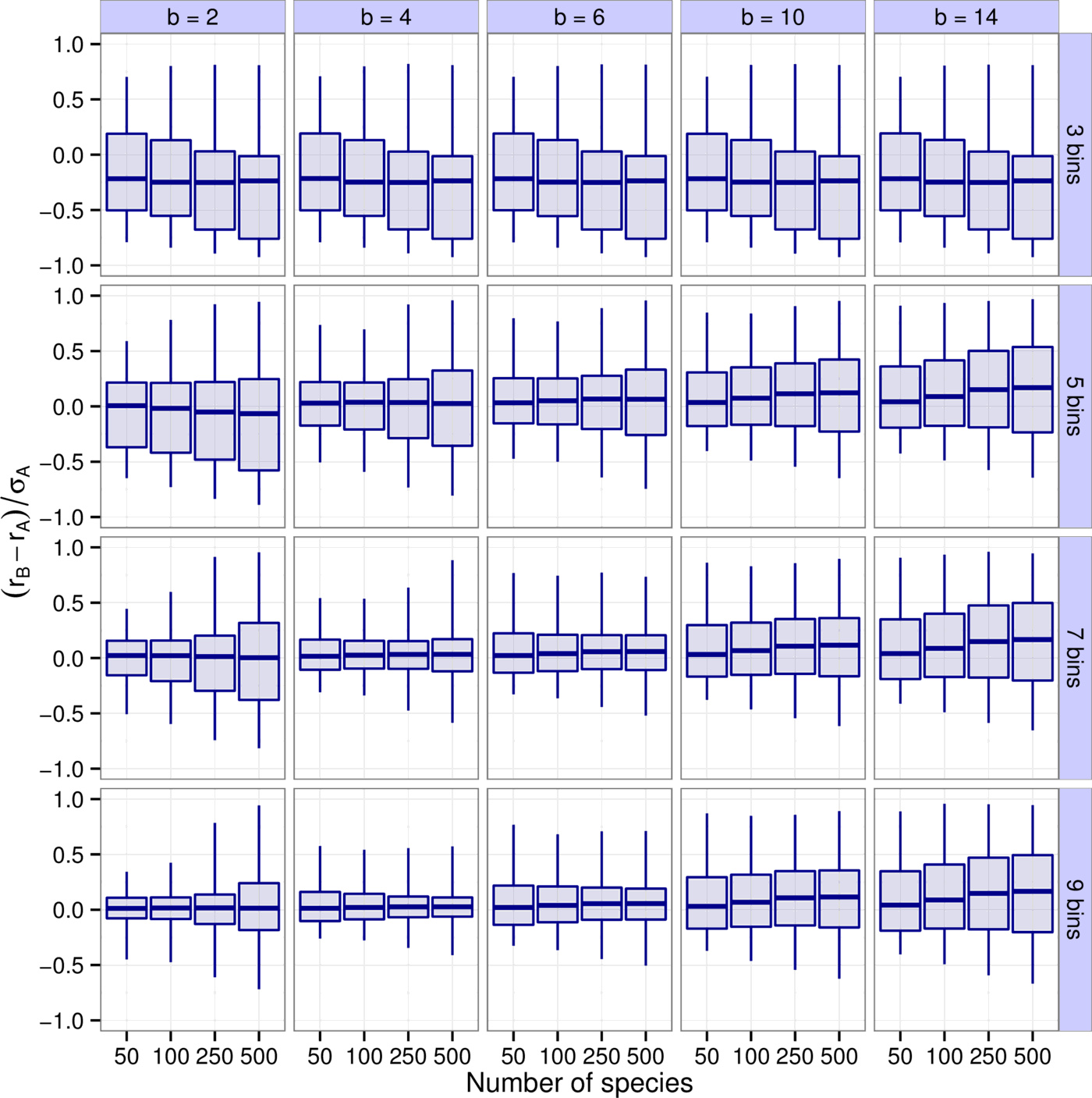
First, we explored how accurately the leading eigenvalue is captured depending on the number of bins $k$, the binning resolution $b$, and the species richness $S$ (Fig. 2). It is apparent that $b=4, \, 6$ and $k=7, \, 9$ yield the best results. For instance, $90\%$ of all results with $b=4$ and $k=7$ have a difference between $r_B$ and $r_A$ less than $16\%$ of $\sigma_A$, the total spread of the real parts of $A$'s eigenvalues. Higher values of $k$ leading to better predictions was expected—the more bins we use, the more accurate the predictions will be. Notice though that there are diminishing returns. In a sense this is fortunate, because using more than 7-9 bins is probably not feasible in practice (seven bins means that, apart from zero, we have a “strong”, a “medium”, and a “weak” category both for positive and negative interactions). The result that $b \approx 4$ is optimal concerns the “best” choice for the definition of an order of magnitude. This suggests one should consider interactions sufficiently different if they differ by a factor of about four. Importantly, this choice proves to be consistently the best through various models and various metrics considered (see the next section and the Supporting Information).
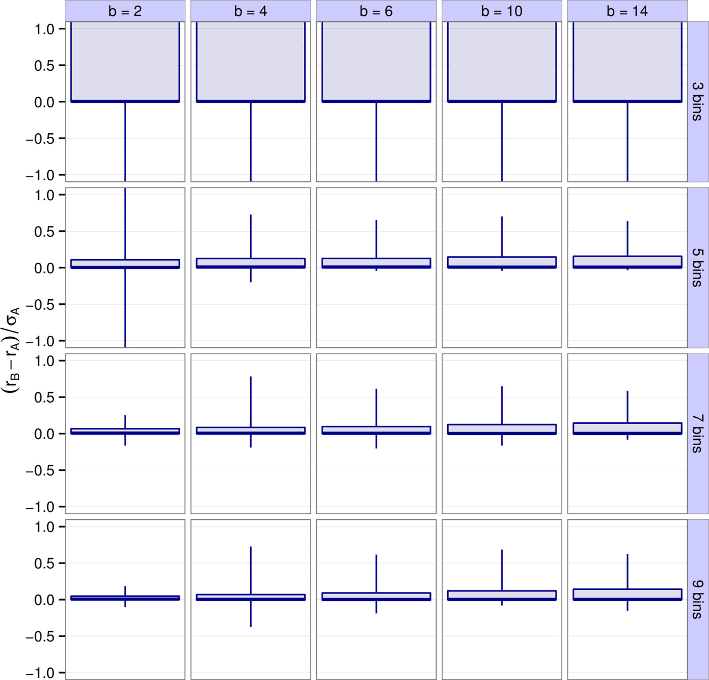
Similarly to the leading eigenvalue, one can also look at reactivity and how well it is predicted (Supporting Information, Figs. S3-S5). Just as before, $b=4, \, 6$ and $k=7, \, 9$ provide the best approximations, with more than $90\%$ of all results falling within $23\%$ of the total spread of the eigenvalues of $H(A)$, the Hermitian part of $A$ (Supporting Information, Figs. S21-S22).
We also consider the effect of changing the connectance on the efficiency of binning—it turns out however that this effect is neither systematic nor very strong (Supporting Information, Figs. S11-S18).
The Allometric Trophic Network
The previous section explored the effects of matrix binning on randomly generated interaction matrices. Here we consider a mechanistic model of multispecies communities, the Allometric Trophic Network [7]. In this model there are a number of noninteracting abiotic resources (here we assume there are two), primary producers utilizing those resources, and consumers eating either the producers or other consumers. The feeding network is generated using the niche model [27]. Consumers interact with their resources via generalized functional responses, which may include consumer interference. These interaction terms are functions of the organisms' average body masses, calculated based on species' trophic levels and simple allometric relationships.
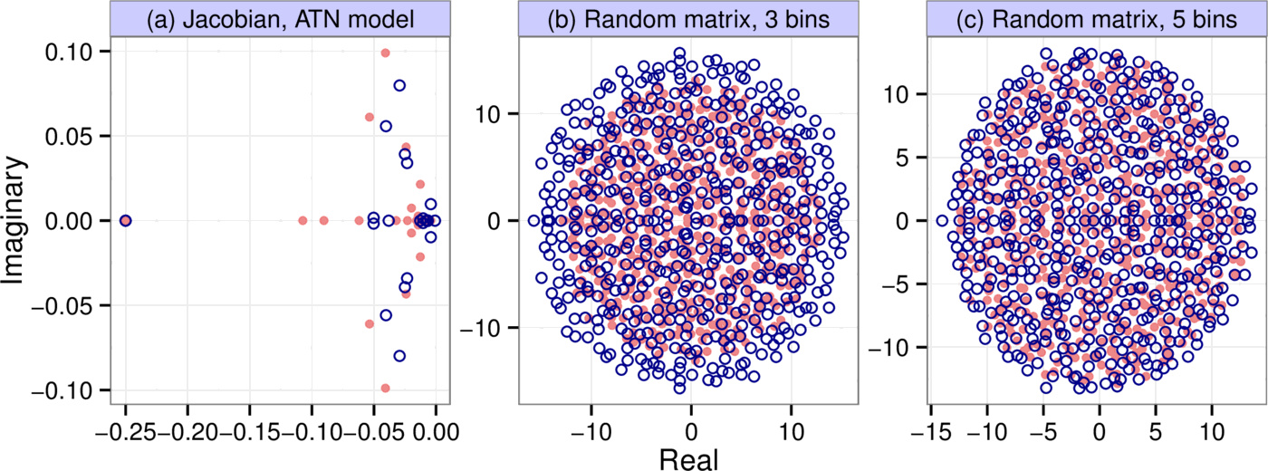
We generated $10,000$ different communities using the Allometric Trophic Network model. In each simulation, we started out from a food web generated by the niche model, with 50 initial species whose abundances were uniformly distributed between $0.05$ and $0.2$. We followed the methodology described in [7] in every aspect to parameterize the model, except in choosing the Hill exponents for the trophic interactions: instead of randomly generating it for every interaction, we assumed it had the constant value of 2. This was done to make the system converge to a fixed point instead of a limit cycle or chaotic attractor, which is important because we are interested in predicting local asymptotic stability (indeed, in our simulations we only ever observed convergence to a fixed point). The model was run until equilibrium was reached, at which point we calculated the Jacobian to obtain the matrix $A$ (see the Supporting Information for a detailed description of our methods). Fig. 3a shows a spectrum generated by the procedure, along with that of its binned counterpart ($b=6$, $k=7$). In the particular simulation shown, 24 species and both abiotic resources survived to stably coexist out of the initial 50 species and two resources. The number of species plus resources persisting at equilibrium was variable between runs, and approximately normally distributed with mean 13.6 and standard deviation 3.0.
Theoretical underpinning
Here we connect the matrix binning procedure with more rigorous mathematical concepts, to give a theoretical underpinning to why and when the method is supposed to work. We employ two arguments, one based on the theory of random matrices, the other on the concept of pseudospectra.
Random matrices
Although empirical interaction webs are manifestly not random, an intuition for why the matrix binning procedure works may be gained by connecting it with random matrix theory [3]. There are several results in the theory of random matrices concerning the distribution of matrix eigenvalues in the complex plane, such as the circular [10] and elliptic [22] laws, which have found ecological applications as well [1]. Here we only consider the simplest version of the circular law; more complexity can be incorporated analogously (see Supporting Information). Suppose the entries of the $S \times S$ matrix $A$ are drawn independently from the same underlying probability distribution $p_A(x)$, which has mean zero and variance $V_A$. Then the law states that for $S$ large, the eigenvalues are uniformly distributed in a circle of radius $\sqrt{S V_A}$ in the complex plane, centered at the origin.
Note that the circle's radius only depends on the variance of $p_A(x)$ but not its shape. This important property [25] means that two completely different underlying probability distributions will lead to the same eigenvalue distribution as long as their mean is zero and their variances are equal (in the limit of $S$ going to infinity, the distributions would converge to be exactly the same; for $S$ large but finite, there are slight but negligible differences). Even if the variances are not equal, the only difference between the eigenvalue distributions will be in the radii of the circles within which the eigenvalues are found.
The key idea concerning matrix binning is as follows. Consider a random matrix $A$ whose entries are drawn from some distribution $p_A(x)$. We create its binned counterpart $B$. But the binned matrix $B$ is just another random matrix with a different underlying probability distribution: we essentially replace the original $p_A(x)$ with a discrete distribution $p_B(x)$, one which we can calculate from $p_A(x)$ and the bin positions. We will then know the eigenvalue distribution of $B$ as well, since that only depends on $p_B(x)$'s variance $V_B$. The spectra of $A$ and $B$ may then be compared analytically.
As an example, let the entries of $A$ come from the uniform distribution $p_A(x) = \mathcal{U}[-1, 1]$, which has variance $V_A = 1 / 3$. Let us bin $A$ with three bins $(-1, \; 0, \; 1)$. The probability, on average, of any one entry being lumped into the $-1$ or $1$ bins is $1/4$, while the probability of being lumped into the $0$ bin is $1/2$, defining the discrete distribution $p_B(x)$. This distribution has variance $V_B = 1 / 2$. The eigenvalues of $A$ are therefore uniformly distributed in a circle of radius $r_A = \sqrt{S / 3}$, and those of $B$ in a circle of radius $r_B = \sqrt{S /2}$ (Fig. 3b). If we now ask how well the leading eigenvalue is approximated, we first note that they are simply given by $r_A$ and $r_B$ (since the eigenvalues fall in a circle). We therefore take the ratio of the two radii to assess the goodness of the approximation: $r_B / r_A = \sqrt{3 / 2} \approx 1.22$. The binned matrix overestimates the leading eigenvalue by this factor.
One could repeat the analysis with a more refined binning scheme, for instance with $k = 5$ and $b = 2$. We then have five bins $(-1, \; -0.5, \; 0, \; 0.5, \; 1)$ instead of the original three, leading to $V_B = 3/8$ (see Supporting Information). Then the ratio of the circles' radii (and that of the leading eigenvalues) is $r_B / r_A = \sqrt{V_B / V_A} = \sqrt{9/8} \approx 1.06$, a near-perfect match brought about by the refinement of the binning resolution (Fig. 3c).
In summary, certain classes of random matrices allow for a simple analytical evaluation of the effects of matrix binning. Although real-world matrices are not going to conform to true random matrices exactly, there are nevertheless good reasons to make use of them anyway. Most importantly, random matrix theory serves as a theoretically well-understood benchmark, a reference model, which, when not fitting real-world data, reveals properties of the empirical system that are causing the departure from the random expectation, thus facilitating a better understanding of the system. Quite apart from this justification, random matrix theory actually does have some success in interpreting empirical data as well [24], suggesting its use may prove more than purely theoretical.
Pseudospectra
The spectrum of a matrix $A$ is the set of complex numbers that are eigenvalues of $A$. In contrast, its $\epsilon$-pseudospectrum [26] is the set of complex numbers that are eigenvalues of all possible perturbed matrices $A + P$, with $\| P \| <\epsilon$ (the matrix norm $\| P \|$ is defined as the square root of the largest eigenvalue of $P^* P$, where $P^*$ is the conjugate transpose of $P$). Whereas the spectrum is composed of discrete points in the complex plane, the $\epsilon$-pseudospectrum comprises of the union of regions of various sizes around the original eigenvalues. See the Supporting Information for an algorithm to compute pseudospectral regions.
An important result [26, Theorem 2.2] states that the $\epsilon$-pseudospectrum of normal matrices (i.e., matrices $A$ for which $A^* A = A A^*$) is the union of circular disks of radius $\epsilon$ around $A$'s unperturbed eigenvalues. Moreover, such matrices have the smallest possible pseudospectra. Any deviation from normality will increase the size of this set, with strongly nonnormal matrices potentially having very large pseudospectral regions even for small values of $\epsilon$.
Pseudospectra provide a rigorous and general measure of the effect of perturbations on the eigenvalues of matrices. Importantly, the binning procedure can be thought of as applying a certain perturbation $P$ to the underlying community matrix $A$, with $A + P = B$, where $B$ is the binned matrix. The pseudospectrum reveals how sensitively the eigenvalues respond to the perturbation induced by binning. In Fig. 5 the blue regions show the $\epsilon$-pseudospectrum for each of the nine empirical webs of Fig. 1, with $\epsilon = \| P \|$ being the appropriate perturbation norm for each web; the red dots are the unperturbed eigenvalues of $A$.
Calculating pseudospectra is straightforward but computationally expensive. In the Supporting Information we therefore introduce a much simpler metric, the scaled departure from normality $\text{depn}(A)$, which characterizes matrix sensitivity with a single number such that $\text{depn}(A) \le 1$ guarantees low sensitivity to perturbations. The value of $\text{depn}(A)$ for each empirical matrix is reported in the panel titles of Fig. 5. All are significantly lower than one, implying their spectra are not sensitive to perturbations—in line with what we see on their pseudospectra.
Discussion
Our results show that certain global community properties, such as stability [15] and reactivity [20], can be predicted using crude, order-of-magnitude estimates of community matrix entries. These properties depend, broadly speaking, on the distribution of eigenvalues (stability depends only on the leading eigenvalue; reactivity on their whole ensemble), which was reasonably captured by the crude approximation. We gave theoretical justification to when and why this would be so, one based on the theory of random matrices, the other on the concept of pseudospectra. To check the robustness of our method, we applied it to three very different scenarios: empirical interaction webs parameterized via allometric relationships [24], randomly generated matrices, and those generated by the Allometric Trophic Network model [7]. Though the degree to which the method produced accurate results was situation-dependent, on the whole, it was able to make reliable predictions in each of these cases.
This predictability appears to be at variance with earlier work emphasizing that even small errors in measuring the entries of the community matrix translate into large errors of prediction [29,30,8,19,21,2]. If the spectrum of the community matrix is well approximated, why would this be the case? The answer, we believe, is that the response of species to press perturbations depends on the inverse spectrum. Due to the preponderance of rare species in natural communities, such systems are necessarily close to a transcritical bifurcation point (small perturbations of the abundances may drive rare species extinct), implying that some eigenvalues are close to zero, making the inverse overly sensitive to measurement errors. One may try to ignore the rare species from a community model, reasoning that—since they are rare—their impact on the community is slight. But unfortunately, due to the general shape of the species-abundance curve [17], there is no natural cutoff point for doing that. Therefore, one should try to approximate properties that do not depend on inverting the community matrix.
One property we have not yet mentioned is feasibility, i.e., whether a community equilibrium has all-positive species abundances. The stability or reactivity of unfeasible equilibria is of no relevance. The reason we did not consider feasibility separately is that we treat the community matrix as the linearization of some arbitrary nonlinear dynamics around some equilibrium state we observe in nature. Its feasibility is therefore already guaranteed by the fact that we are observing the system. Apart from this, note that feasibility is a property that depends on the inverse problem. For instance, in a simple Lotka–Volterra model given by $\mathrm{d} n /\mathrm{d} t = n \circ \left( b + An \right)$ (where $n$ is the vector of densities, $b$ the vector of intrinsic growth rates, $A$ the matrix of interaction coefficients, and $\circ$ denotes the Hadamard or element-by-element product), the equilibrium densities are given by $n = -A^{-1} b$. Therefore, as discussed, our method is ill-suited for determining feasibility to begin with.
The accuracy of prediction was dependent on the number of bins $k$ the entries were classified into (fewer bins meant larger errors), and on the choice of the binning resolution $b$. In practice, a $k$ of seven to nine is probably the largest feasible number, since beyond this it becomes increasingly difficult to assign weak interactions to correct bins. For the binning resolution $b$, we found that values beyond $10$ gave significantly worse results; $b\approx 4$ was usually optimal, but the sensitivity of the results was not very great, and $b=2$ and $b=6$ performed similarly (Figs. 2, 4, S4, S9). Interestingly, we have found $b \approx 4$ to perform the best regardless of whether we looked at the empirical data, the randomly generated webs, or the Allometric Trophic Networks, and regardless of whether we estimated stability or reactivity.
It may seem counterintuitive that the smallest value of $b$ is not the most accurate in recovering matrix properties. After all, the finer the resolution, the more accurate the binning. The reason is that, because the number of bins is finite, this finer resolution only applies to larger matrix entries but not necessarily to smaller ones. Consider the following example. A $100 \times 100$ matrix is generated by uniformly sampling all but two of its entries from $[-2, \; 2]$, and then setting the remaining two entries to $-8$ and $8$, respectively. If we bin this matrix with $b = 2$ and $k = 5$, the bins are $(-8, \; -4, \; 0, \; 4, \; 8)$. This means that all but the two outliers will be classified in the binned matrix as zero—a crude estimate if there ever was one. However, for $b = 4$ the bins become $(-8, \; -2, \; 0, \; 2, \; 8)$, resolving the underlying data much better. In the end, the best binning is, of course, achieved for $b \rightarrow 0$ and $k \rightarrow \infty$. Since this is not feasible in practice, one has to find the best compromise between a $b$ that is not too large but cannot be too small, and a $k$ that is not too small but cannot be too large.
We also checked what happens if, in estimating the strongest interactions $p$ and $n$, we use $10$ empirically measured results and take their average. This way, a single very strong interaction that dominates the system will not artificially distort the binning. However, the results proved insensitive to doing this. The implication is that one should concentrate expensive and time-consuming empirical effort wisely: very accurate measurement of a couple of interaction coefficients does not improve predictive power much, while qualitative knowledge of many matrix entries does.
It is easy to think of scenarios in which the binning procedure produces grossly inaccurate results. For instance, we have seen that matrices with $\text{depn}(A) \gg 1$ will have sensitive spectra, therefore even relatively slight perturbations of their entries (e.g. introduced by binning) may lead to large changes in their eigenvalue structure. We emphasize however that our metric for the scaled departure from normality is merely a proxy for matrix sensitivity: the complete picture is gained by looking at the full pseudospectrum.
But the binning procedure may be inaccurate even when the degree of nonnormality is low. If the interaction strengths span too many orders of magnitude or are dominated by a small number of very large matrix entries, then even a reasonably fine-grained binning structure may classify all but the handful of very large entries as zero, leading to an eigenvalue distribution wildly different from the actual one. The reason why low nonnormality does not matter in this case is that the perturbation induced by binning is in fact very large. In practice however, whenever a few interactions dominate the system, instead of binning, one should concentrate just on those very large entries to gain insight into its workings. In other words, such systems naturally require different methods of analysis than the one presented here, which works better for complex interaction structures where many interactions together shape the properties of the system.
Our results also shed light on the classic stability-complexity debate from a slightly different angle. The original “conventional wisdom” was that more complex systems (i.e., ones with more species, higher variance in the strength of interactions, and higher connectance) would be more stable in the face of perturbations [5, p. 586]. This view was challenged by the classic result of [14] which argued that, all else being equal, more complex systems have a lower probability of being stable: the eigenvalues of the community matrices of more complex systems are less likely to reside in the left half of the complex plane. Whether May's argument actually poses a true challenge to the conventional wisdom has been heavily debated [16]. Our findings contribute to this debate by showing that large, complex systems, if not necessarily more stable, are very robust against perturbations of the community matrix entries. The binning of a matrix can be thought of as a structural perturbation of the system: we are altering the matrix entries, changing the strength of interactions between species. Since, as we have seen, the binning of large complex interaction matrices has only a small effect on the spectrum, the perturbation induced by binning does not have a large effect on the system's large-scale properties. For instance, the stability and reactivity properties were unchanged. This means that if the system was actually stable, it was likely to stay that way, and conversely, unstable systems remained unstable after the perturbation induced by binning. In fact, the robustness interpretation of the stability-complexity debate is closer to its original formulation, where it was argued that the more pathways there are in an interaction web, the less it matters if one of those links is lost, since other pathways will compensate for the loss [13].
In summary, the results from approximating system properties using semiquantitative information point in the direction of using such approximations in practice, where obtaining precise quantitative information is hard, expensive, and time-consuming. The presented results show that such crude parameterization of complex systems may still reveal important global system properties of interest.
Acknowledgements
We thank A. Golubski, J. Grilli, M. J. Michalska-Smith, and E. L. Sander for discussions, and B. Althouse and four anonymous reviewers for their helpful comments. This work was supported by NSF #1148867.
References
- Allesina, S., Tang, S., 2012. Stability criteria for complex ecosystems. Nature 483, 205–208.
- Aufderheide, H., Rudolf, L., Gross, T., Lafferty, K. D., 2013. How to predict community responses to perturbations in the face of imperfect knowledge and network complexity. Proceedings of the Royal Society of London Series B 280, 20132355.
- Bai, Z., Silverstein, J. W., 2009. Spectral analysis of large dimensional random matrices. Springer.
- Barabás, G., Pásztor, L., Meszéna, G., Ostling, A., 2014. Sensitivity analysis of coexistence in ecological communities: theory and application. Ecology Letters 17, 1479–1494.
- Begon, M., Townsend, C. R., Harper, J. L., 2005. Ecology: From Individuals to Ecosystems. {F}ourth edition. Blackwell Science Publisher, London.
- Bender, E. A., Case, T. J., Gilpin, M. E., 1984. Perturbation experiments in community ecology: Theory and practice. Ecology 65, 1–13.
- Berlow, E. L., Dunne, J. A., Martinez, N. D., Stark, P. B., Williams, R. J., Brose, U., 2009. Simple prediction of interaction strengths in complex food webs. Proceedings of the National Academy of Sciences USA 106, 187–191.
- Dambacher, J. M., Li, H. W., Rossignol, P. A., 2002. Relevance of community structure in assessing indeterminacy of ecological predictions. Ecology 83, 1372–1385.
- Elton, C. S., 1958. The Ecology of Invasions by Animals and Plants. Methuen, London.
- Girko, V. L., 1984. The circle law. Theory of Probability and its Applications 29, 694–706.
- Levins, R., 1968. Evolution in changing environments. Princeton University Press, Princeton.
- Levins, R., 1974. Qualitative analysis of partially specified systems. Ann. NY Acad. Sci. 231, 123–138.
- MacArthur, R. H., 1955. Fluctuations of animal populations and a measure of community stability. Ecology 36, 533–536.
- May, R. M., 1972. Will a large complex system be stable? Nature 238, 413–414.
- May, R. M., 1973. Stability and Complexity in Model Ecosystems. Princeton University Press, Princeton.
- McCann, K. S., 2000. The diversity-stability debate. Nature 405, 228–233.
- McGill, B. J., Etienne, R. S., Gray, J. S., Alonso, D., Anderson, M. J., Benecha, H. K., Dornelas, M., Enquist, B. J., Green, J. L., He, F., Hurlbert, A. H., Magurran, A. E., Marquet, P. A., Maurer, B. A., Ostling, A., Soykan, C. U., Ugland, K. I., White, E. P., 2007. Species abundance distributions: moving beyond single prediction theories to integration within an ecological framework. Ecology Letters 10, 995–1015.
- Meszéna, G., Gyllenberg, M., Pásztor, L., Metz, J. A. J., 2006. Competitive exclusion and limiting similarity: a unified theory. Theoretical Population Biology 69, 68–87.
- Montoya, J. M., Woodward, G., Emmerson, M. C., Solé, R. V., 2009. Press perturbations and indirect effects in real food webs. Ecology 90, 2426–2433.
- Neubert, M. G., Caswell, H., 1997. Alternatives to resilience for measuring the responses of ecological systems to perturbations. Ecology 78, 653–665.
- Novak, M., Wootton, J. T., Doak, D. F., Emmerson, M., Estes, J. A., Tinker, M. T., 2011. Predicting community responses to perturbations in the face of imperfect knowledge and network complexity. Ecology 92, 836–846.
- Sommers, H. J., Crisanti, A., Sompolinsky, H., Stein, Y., 1998. Spectrum of large random asymmetric matrices. Physical Review Letters 60, 1895–1898.
- Tang, S., Allesina, S., 2014. Reactivity and stability of large ecosystems. Frontiers in Ecology and Evolution. \newline\urlprefixhttp://dx.doi.org/10.3389/fevo.2014.00021
- Tang, S., Pawar, S., Allesina, S., 2014. Correlation between interaction strengths drives stability in large ecological networks. Ecology Letters 17, 1094–1100.
- Tao, T., Vu, V., Krishnapur, M., 2010. Random matrices: Universality of esds and the circular law. Annals of Probability 38 (5), 2023–2065.
- Trefethen, L. N., Embree, M., 2005. Spectra and Pseudospectra: The Behavior of Nonnormal Matrices and Operators. Princeton University Press, New Jersey, USA.
- Williams, R. J., Martinez, N. D., 2000. Simple rules yield complex food webs. Nature 404, 180–183.
- Woodward, G., Speirs, D. C., Hildrew, A. G., 2005. Quantification and resolution of a complex, size-structured food web. Advances in Ecological Research 36, 85–135.
- Yodzis, P., 1988. The indeterminacy of ecological interactions as perceived through perturbation experiments. Ecology 69, 508–515.
- Yodzis, P., 2000. Diffuse effects in food webs. Ecology 81, 261–266.
Footnotes
1. Let $A$ be a normalized matrix, with entries having zero mean and unit variance. Denote its eigenvalues by $\lambda_A$ and their variance by $\text{Var}(\lambda_A)$. Now let $B = \alpha A$ with $\alpha > 0$ a scaling constant. $B$'s entries then have zero mean and variance $\alpha^2$, its eigenvalues are $\lambda_B = \alpha \lambda_A$, and their variance is $\text{Var}(\lambda_B) = \text{Var}(\alpha \lambda_A) = \alpha^2 \text{Var}(\lambda_A)$. In other words, increasing/decreasing the variance of the matrix entries increases/decreases the variance of the eigenvalues as well.